OUTLINE -- LESSONS 3a, 3b, 3c
Understanding Individual Markets: Demand and Supply
Parts of this lecture can be found at:
http://www.harpercollege.edu/mhealy/eco211/lectures/microch3-17.htm
|
Additional Web Pages for this lecture:
|
|
The type of news articles that pertain to this
chapter:
|
I. Introduction: Prices and the 5Es
- From what we know about the 5
Es of economics, why are we studying PRICES?
- Prices are important to achieve which of the Es?
- In a Capitalist Economic System (Lesson
2a), Prices are the result of the interaction of Supply
and Demand
- Preview:
- If the price of pizza increase, what happens to the
demand for pizza?
- If the price of plywood increases what happens to the
supply of plywood?
II. Demand
A. Definition
1. a schedule
2. various quantities
3. willing and able
4. various prices
5. given time period
6. ceteris paribus
7. demand is NOT how much we buy
B. Demand Schedule and Curve [sdtabblk.gif]
[sdpoint.gif]
[sdline.gif]
C. Law of Demand
1. there is an inverse relationship between price
and quantity demanded
2. why?
a. common sense
b. diminishing marginal utility
c. income effect
d. substitution effect
D. Market Demand
1. definition
2. graphically
E. Determinants of Demand (VODKA)
1. the price of the
product
2. the non-price determinants of
demand
V. Two Kinds of Changes Involving Demand
A. Change in Quantity Demanded
1. caused ONLY by a change in the PRICE of the
product
2. a movement ALONG a SINGLE demand curve
B. Change in Demand
1. shifting the demand curve / a new demand
schedule
a. an increase in demand
b. a decrease in demand
2. caused by a CHANGE in the non-price determinants of
demand
a. Pe -- expected price
b. Pog -- price of other goods
1) substitute goods
2) complementary goods
3) independent goods
c. I -- income
1) normal goods
2) inferior goods
d. N -- number of POTENTIAL consumers
1) population change
2) expanded marketing area
3) new competitor
(changes individual demand curve but NOT market demand
curve)
4) change in eligible consumers (i.e. drinking age)
e. T -- tastes and preferences
III. Supply
A. Definition
1. a schedule
2. various quantities
3. willing and able
4. various prices
5. given time period
6. ceteris paribus
7. supply is NOT the quantity available for sale
B. Supply Schedule and Curve sssupply.gif
sdspnt.gif
sdsline.gif
C. Law of Supply
1. there is a direct relationship between price and
quantity supplied
2. why?
a. common sense
b. increasing costs because some resources are fixed
c. increasing costs because not all resources are
identical
D. Market Supply
E. Determinants of Supply
1. the price of the product
2. the non-price determinants of supply
VI. Two Kinds of Changes Involving
Supply
A. Change in Quantity Supplied schgqs.gif
1. caused ONLY by a change in the PRICE of the
product
2. a movement ALONG a SINGLE supply curve
B. Change in Supply slineinc.gif
1. shifting the supply curve / a new supply
schedule
a. an increase in supply
b. a decrease in supply
2. caused by a CHANGE in the non-price determinants of
supply
a. Pe -- expected price
b. Pog -- price of other goods ALSO PRODUCED BY THE FIRM
c. Pres -- price of resources
d. T --technology
e. T --taxes and subsidies
f. N -- number of sellers
3c - Market Equilibrium and
Efficiency
|
IV. Market Equilibrium -- Equilibrium Price
and Quantity
A. Market Equilibrium
1. define equilibrium
2. find market equilibrium sdequil.gif
B. Market Disequilibrium
1. surpluses
2. shortages
What causes prices to
change?
|
VII. Changes in Demand AND
Supply
A. Case 1: D changes and supply stays the same
dinc.gif
B. Case 2: S changes and demand stays the same sinc.gif
C. Case 3: D and S both change
1. S increases, D decreases
2. S decreases, D increases SDdisd.gif
3. S increases, D increases SDdisi.gif
4. S decreases, D decreases
VIII. Examples:
- Chapter Appendix: Additional Examples of Supply
and Demand
- I. Changes in Supply and Demand
A. Lettuce
B. Exchange Rates
- 1. One of the largest foreign exchange
markets is the euro-dollar market.
2. The price of a euro is expressed in
dollars and is determined by demand and supply of
euros.
3. U.S. firms require euros to buy goods from
European countries and this is reflected by the
demand for euros.
4. When European countries buy goods from the
U.S. they must convert euros to dollars thereby
creating the supply of euros.
5. Increased popularity of European goods in
the U.S. increases the demand for euros, causing
equilibrium price to increase and the dollar
depreciates while the euro
appreciates.
C.Pink Salmon
- 1. This is an example of simultaneous
changes in both supply and demand.
2. An increase in supply occurs because of
more efficient fishing boats, the development of
fish farms, and new entrants to the
industry.
3. There is a decrease in demand because of
changes in consumer preference, and an increase in
income shows pink salmon to be an inferior
good.
4. Both changes put downward pressure on the
price of pink salmon. Because we know that the
increase in supply of pink salmon exceeded the
decrease in demand, we can also determine that the
quantity purchased increased.
D. Gasoline
- 1. U.S. gas prices have rapidly increased
over the past few years.
2. Middle East politics and military
conflicts (both real and anticipated) have
disrupted supply, tending to drive gas prices
up.
3. Increased popularity of SUVs and other
low-gas-mileage vehicles has increased the demand
for gas, also tending to drive the price
up.
4. While theoretically the affect on quantity
is indeterminate, in reality the quantity purchased
has increased, suggesting that the increase in
demand exceeded the decrease in
supply.
E. Sushi
- 1.Despite fast-growing popularity of sushi
bars in the United States, prices have remained
relatively constant.
2.The increase in demand can be attributed to
an increased taste for sushi.
3.The opening of sushi bars in response to
expected and realized demand has increased the
supply of sushi, helping to keep the price
stable.
II. Preset Prices
|
IX. The Market System and Efficiency
See: YELLOW PAGES: The supply and demand
model and allocative efficiency
A. Introduction: The Market System and Efficiency
A. Equilibrium price and allocative efficiency
B. Two models
a. MB = MC (MSB = MSC)
b. Consumer and producer surplus
B. The MB=MC model
1. WHAT WE GET:
a. Goal of businesses: Maximize Profits
b. Therefore, they will produce where:
- the Market Equilibrium quantity
- the quantity where Qs=Qd
- the is "what we get"
- Graphically:
c. Assumptions: pure capitalism
2. WHAT WE WANT: ALLOCATIVE EFFICIENCY
a. Review :
(1) Allocative Efficiency
definition - using our limited resources
to produce:
- The quantity of goods and services that
maximizes society's satisfaction
- using resources to produce more CDs that
people want and fewer cassette tapes that they
don't want
- no shortages and no surpluses
(2) Benefit-Cost Analysis
definition -
the selection of ALL possible
alternatives where the marginal benefits are
greater than the marginal cost
select all where: MB >
MC
up to where: MB = MC
but never where: MB < MC
3. Allocative Efficiency is achieved where:
a. MSB=MSC
1) define Marginal Social Benefits (MSB)
2) define Marginal Social Costs (MSC)
3) therefore if society gets
all quantities
where: MSB > MSC
up to where: MSB = MSC
but never where: MSB < MSC
this will be the
quantity where society's Satisfaction will be
maximized or the allocatively efficient
quantity
b. Graphically:
4. THEREFORE:
a. Businesses will produce the profit maximizing
or market equilibrium quantity - the quantity where
Qd=Qs
b. Society wants the allocatively efficient quantity -
the quantity where MSB=MSC
c. WHAT WE GET = WHAT WE WANT if:
1) Market Demand = Marginal Social Benefits
(D=MSB)
a) law of diminishing marginal utility
b) assuming no positive externalities (no spillover
benefits) D=MSB
2) Market Supply = Marginal Social Costs
(S=MSC)
a) law of increasing costs
b) assuming no negative externalities (no spillover
costs) S=MSC
5. Competitive Markets and Allocative Efficiency
(MSB=MSC)
a. if there are no negative externalities (no
spillover costs,) then S = MSC,
b. if there are no positive externalities (no
spillover benefits), then D = MSB,
c. Graphically:
d. Then: WHAT WE GET = WHAT WE WANT and market
economies achieve allocative efficiency
|
In a market economy with no spillover
benefits and no spillover costs:
the profit maximizing
or market equilibrium quantity
(what we get)
WILL BE THE SAME AS
the allocative efficient
quantity
(what we want)
|
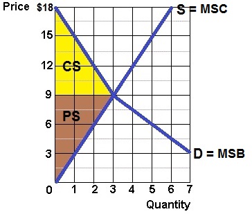
C. Consumer and Producer Surplus Model to show why the
equilbrium price maximizes society's satisfaction
1. Consumer Surplus
a. definition
- the difference between the maximum price a
consumer is (or consumers are) willing to pay for a
product and the actual price.
- The surplus, measurable in dollar terms, reflects
the extra utility gained from paying a lower price than
what is required to obtain the good.
c. graph
- Consumer surplus (CS) is measured and represented
graphically by the area under the demand curve and above
the equilibrium price.

-
c. calculate
- Consumer surplus can be measured by calculating
the difference between the maximum willingness to pay and
the actual price for each consumer, and then summing
those differences.

- d. Consumer surplus and price are inversely related -
all else equal, a higher price reduces consumer
surplus.
2. Producer Surplus
a. definition
- the difference between the actual price a producer
receives (or producers receive) and the minimum
acceptable price.
b. graph
- Producer surplus (PS) is measured and represented
graphically by the area above the supply curve and below
the equilibrium price.

c. calculate
- Producer surplus can be measured by calculating
the difference between the minimum acceptable price and
the actual price for each unit sold, and then summing
those differences.

d. Producer surplus and price are directly related -
all else equal, a higher price increases producer
surplus
3. Efficiency at equilibrium
a. Efficiency is attained at equilibrium, where
the combined consumer and producer surplus is maximized.

- Consumers receive utility up to their maximum
willingness to pay, but only have to pay the equilibrium
price.
- Producers receive the equilibrium price for each
unit, but it only costs the minimum acceptable price to
produce.
b. Allocative efficiency occurs at quantity levels
where three conditions exist:
- MB = MC (MSB = MSC)
- maximum willingness to pay = minimum acceptable
price
- combined consumer and producer surplus is at a
maximum
4. Allocative Inefficiency (Deadweight Losses)
a. producing too little:
- underproduction reduces both consumer and producer
surplus, and efficiency is lost because both buyers and
sellers would be willing to exchange a higher
quantity.
- the efficiency loss (deadweight loss) of producing
too little is the brown triangle on the figure below
- The sum of producer and consumer surplus at the
equilibirum level of output was the triangle
abc
- at the lower level of output the sum of
consumer and producer surplus is adec
- so the efficiency loss of producing too little
is the brown triangle dbe
- between Q2 and Q1 the maximum willingness to
pay of consumers is above the minimum acceptable price
of seller
b. producing too much:
- overproduction causes inefficiency because past
the equilibrium quantity, it costs society more to
produce the good than it is worth to the consumer in
terms of willingness to pay.
- the efficiency loss (deadweight loss) of producing
too little is the tan triangle on the figure below
- at the higher level of output the efficiency
loss caused by producing too much (Q3) is the tan
triangle bfg
- between Q1 and Q3 the maximum willingness to
pay of consumers is below the minimum acceptable price
of seller, this subtracts from society's net
benefit


Efficiency loss from underproduction = c + d

Efficiency loss from underproduction = e + f