A. Equilibrium price and allocative efficiencyB. Two models
a. MB = MC (MSB = MSC)b. Consumer and producer surplus
B. The MB=MC model
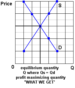
1. WHAT WE GET:a. Goal of businesses: Maximize Profits
b. Therefore, they will produce where:
- the Market Equilibrium quantity
- the quantity where Qs=Qd
- the is "what we get"
- Graphically:
c. Assumptions: pure capitalism
2. WHAT WE WANT: ALLOCATIVE EFFICIENCY
a. Review :(1) Allocative Efficiencydefinition - using our limited resources to produce:
- The quantity of goods and services that maximizes society's satisfaction
- using resources to produce more CDs that people want and fewer cassette tapes that they don't want
- no shortages and no surpluses
(2) Benefit-Cost Analysis
definition -the selection of ALL possible alternatives where the marginal benefits are greater than the marginal costselect all where: MB > MC
up to where: MB = MC
but never where: MB < MC3. Allocative Efficiency is achieved where:
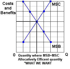
a. MSB=MSC1) define Marginal Social Benefits (MSB)2) define Marginal Social Costs (MSC)
3) therefore if society gets
all quantities where: MSB > MSC
up to where: MSB = MSC
but never where: MSB < MSCthis will be the quantity where society's Satisfaction will be maximized or the allocatively efficient quantity
b. Graphically:
4. THEREFORE:
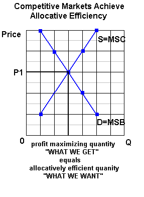
a. Businesses will produce the profit maximizing or market equilibrium quantity - the quantity where Qd=Qsb. Society wants the allocatively efficient quantity - the quantity where MSB=MSC
c. WHAT WE GET = WHAT WE WANT if:
1) Market Demand = Marginal Social Benefits (D=MSB)a) law of diminishing marginal utility
b) assuming no positive externalities (no spillover benefits) D=MSB2) Market Supply = Marginal Social Costs (S=MSC)
a) law of increasing costs
b) assuming no negative externalities (no spillover costs) S=MSC5. Competitive Markets and Allocative Efficiency (MSB=MSC)
a. if there are no negative externalities (no spillover costs,) then S = MSC,b. if there are no positive externalities (no spillover benefits), then D = MSB,
c. Graphically:
d. Then: WHAT WE GET = WHAT WE WANT and market economies achieve allocative efficiency
In a market economy with no negative or positive externalities:
(no spillover benefits and no spillover costs)the profit maximizing or market equilibrium quantity
(what we get)WILL BE THE SAME AS
the allocative efficient quantity
(what we want)
C. Consumer and Producer Surplus Model to show why the equilibrium price maximizes society's satisfaction (pp. 126-129)
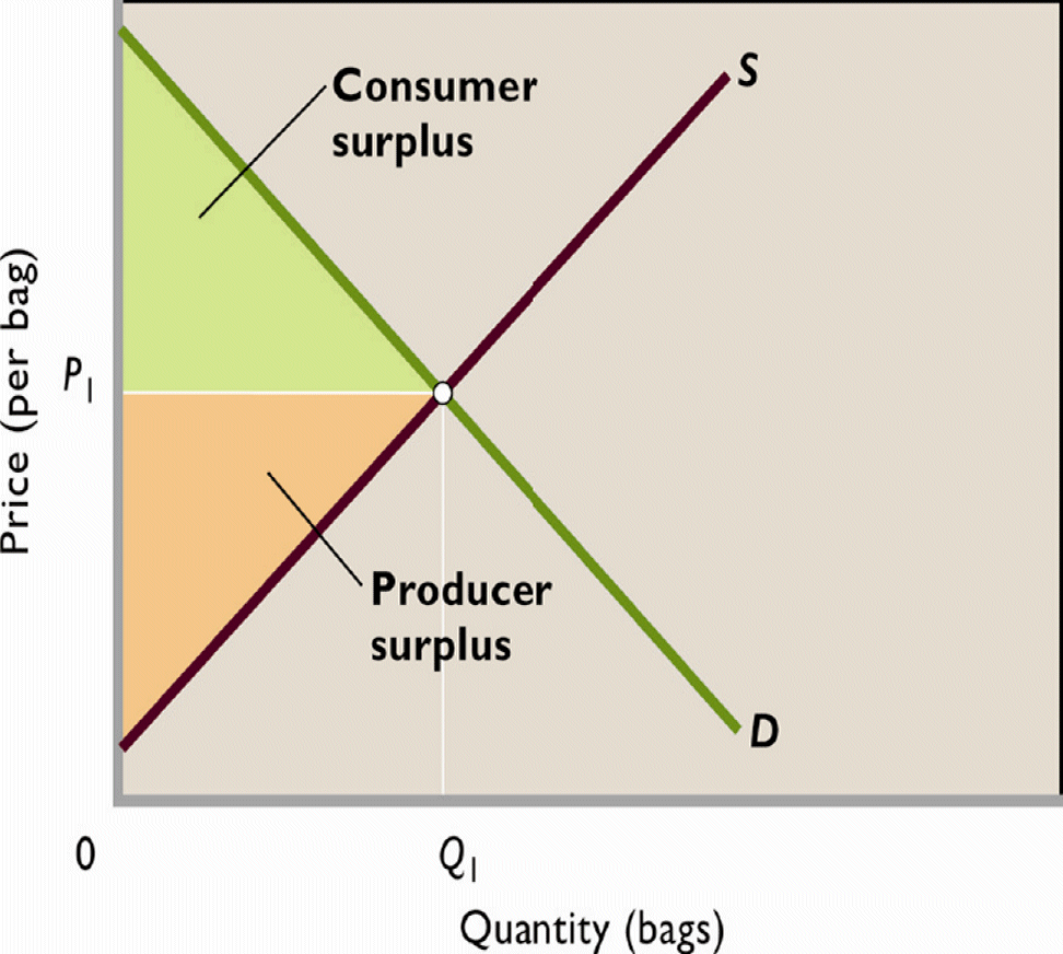
1. Consumer Surplus (figure 6.5 and table 6.5)a. definition: the difference between the maximum price a consumer is (or consumers are) willing to pay for a product and the actual price.b. The surplus, measurable in dollar terms, reflects the extra utility gained from paying a lower price than what is required to obtain the good.
c. graph
Consumer surplus is measured and represented graphically by the area under the demand curve and above the equilibrium price.
d. calculate
Consumer surplus can be measured by calculating the difference between the maximum willingness to pay and the actual price for each consumer, and then summing those differences.
e. Consumer surplus and price are inversely related - all else equal, a higher price reduces consumer surplus.
2. Producer Surplus (figure 6.6 and table 6.6)
a. definition: the difference between the actual price a producer receives (or producers receive) and the minimum acceptable price.
b. graph
Producer surplus is measured and represented graphically by the area above the supply curve and below the equilibrium price.
c. calculate
Producer surplus can be measured by calculating the difference between the minimum acceptable price and the actual price for each unit sold, and then summing those differences.
d. Producer surplus and price are directly related - all else equal, a higher price increases producer surplus
3. Efficiency at equilibrium (figure 6.7)
a. Efficiency is attained at equilibrium, where the combined consumer and producer surplus is maximized. (Figure 6.7)
Consumers receive utility up to their maximum willingness to pay, but only have to pay the equilibrium price.
Producers receive the equilibrium price for each unit, but it only costs the minimum acceptable price to produce.
b. Allocative efficiency occurs at quantity levels where three conditions exist:
MB = MC (MSB = MSC)
maximum willingness to pay = minimum acceptable price
combined consumer and producer surplus is at a maximum
4. Allocative Inefficiency (Deadweight Losses [Figure 6.8])
a. producing too little:underproduction reduces both consumer and producer surplus, and efficiency is lost because both buyers and sellers would be willing to exchange a higher quantity.
the efficiency loss (deadweight loss) of producing too little is the brown triangle on the figure below
The sum of producer and consumer surplus at the equilibrium level of output was the triangle abcat the lower level of output the sum of consumer and producer surplus is adec
so the efficiency loss of producing too little is the brown triangle dbe
between Q2 and Q1 the maximum willingness to pay of consumers is above the minimum acceptable price of seller
b. producing too much:
overproduction causes inefficiency because past the equilibrium quantity, it costs society more to produce the good than it is worth to the consumer in terms of willingness to pay.
the efficiency loss (deadweight loss) of producing too little is the tan triangle on the figure below
at the higher level of output the efficiency loss caused by producing too much (Q3) is the tan triangle bfgbetween Q1 and Q3 the maximum willingness to pay of consumers is below the minimum acceptable price of seller, this subtracts from society's net benefit


