Unit 1: Markets are Efficient, Except
. . . Intro to Microeconomics
Lesson 1a: The Class and the
Math
Welcome to ECO 211! My name is Mark Healy. I
will be your economics instructor for the semester. Please call me
"Mark".
Many students end up dropping or failing this
course due to the lack of basic math skills. If your math skills are
weak you should consider building them before taking this course. If
you are required to take MTH 060 or MTH 082 and have not yet done so,
do not take this economics course until you have successfully
completed one of them. I have posted a practice math quiz on our
Blackboard site. Please take the 20 question math quiz. If you score
less than 14 or 15, consider dropping ECO 211 and taking a math class
first. Contact your instructor if you have questions or
concerns.
This course will cover the area of economics
commonly defined as MICROECONOMICS which is concerned with the
individual parts of the economy such as individual businesses or
industries, individual consumers, and individual products. Our goal
is to study whether the economy uses our limited resources to obtain
the maximum satisfaction possible for society. We will concentrate on
three issues or goals: ALLOCATIVE EFFICIENCY, PRODUCTIVE EFFICIENCY,
and EQUITY.
1a Something Interesting - Why are we
studying this?
|
Optional: a funny look at some major
ideas of economics by the "Stand-up Economist".
Principles
of economics, translated
(5:20)
pp. 24-28, (19th, pp. 22-26) "Graphs and Their
Meaning"
Syllabus
On-Campus / Syllabus
Online
Start: 5Es
online reading
Lecture
Outline
1a Assignments: Video
Lectures
|
REVIEW OF GRAPHING CONCEPTS
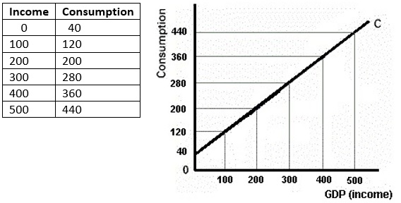
1.2.1 Using
Graphs to Understand Direct Relationships
9:50 [MyNotes]
1.2.2
Plotting
A Linear Relationship Between Two Variables
9:57 [MyNotes]
1.2.3
Changing
the Intercept of a Linear Function
8:42 [MyNotes]
1.2.4
Understanding
the Slope of a Linear Function 7:28
[MyNotes]
OPTIONAL:
Khan Academy Exercise:
Graphing
Points
Khan
Academy Exercise: Graphing
Points 2
OPTIONAL:
MATH, ALGEBRA, AND GEOMETRY FOR ECONOMICS STUDENTS
How
to Multiply and Divide Fractions in Algebra for
Dummies (YouTube fordummies
1:50)
Simple
Equations (Khan Academy
11:06)
Solving
One-Step Equations (Khan Academy
1:54)
Solving
One-Step Equations 2 (Khan Academy
2:23)
Practice
(Khan Academy )
Solving
Ax + B = C (Khan Academy
8:41)
Area
and Perimeter (Khan Academy 8:24 -
begin at 3:55)
1a Outcomes - What you should
learn
|
How to find class information:
- Syllabus
- Blackboard
- Yellow Pages
- SCHEDULE
- LESSONS webpage
- MICWEBAPP
- Key Term Flashcards
- Web Quizzes
- Key Problems
Basic math skills:
- calculate marginal
- calculate average
- arithmetic of fractions and
decimals
- find area of a rectangle
- find area of a triangle
- basic algebra
- calculate and use percentages
- graph a line on a Cartesian coordinate
system
- marginal is the slope of the
total
- total equals the area under the
marginal
Key Terms
Flash Cards - Click Here
The Class:
Required Activity, Yellow Pages,
Tomlinson Videos on Thinkwell, Video Notes, LESSONS webpage,
Pre-quiz, Clicker Quiz, Web Quiz,
The Math:
horizontal (x) axis, vertical (y)
axis, origin, direct (positive) relationship, inverse (negative)
relationship, slope of a line, positive slope, negative slope,
marginal, average
Slope = rise/run
Slope = vertical change / horizontal change
Slope = marginal value of the total
Marginal = change in total / change in
quantity
The area under a marginal curve = the
total
Average = total / quantity
Total = average x quantity
Total = the sum of the marginal
Total = the area under the marginal
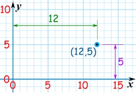
Any Point on a Graph Represents Two
Numbers
Direct Relationship
Inverse Relationship
Calculating Slope
The area under a marginal curve = the
total
Episode
5A: Models & Theories
[3:26 YouTube mjmfoodie]
Episode
6: Graph Review
[4:22 YouTube mjmfoodie]
NOTE: These are REVIEW videos only. In order to
learn the material you must read the assigned textbook readings,
watch the assigned lecture videos, and do problems. See the
MICWEBAPP
or the LESSONS
link for these assignments.
Unit 1: Markets are Efficient, Except
. . . Intro to Microeconomics
Lesson 1b: The 5Es of
Economics
The "5Es of Economics" are not from the
textbook. I borrowed the concept (with many modifications) from
another textbook many years ago. I believe it concisely explains the
purpose of economics. Also, it begins to introduce students to the
economic way of thinking. The economic problem that we all face, that
all countries face, that the world faces, is SCARCITY. Economics is
the study of how we can reduce scarcity. What I like about the 5Es
model is that it shows us that there are only five ways to reduce
scarcity. Only five. I call them the "5Es" of economics.
The "5Es" of Economcs are:
1. Economic Growth
2. Allocartive Efficiency
3. Productive Efficiency
4. Equity
5. Full Employment
For each of the 5Es:
1. learn the definition,
2. understand examples, and,
3. most importantly, know how they reduce scarcity and help to
increase society's satisfaction.
This is where you learn that it may be good
when the price of plywood increases greatly as the result of a
hurricane. And why it might be good when Coca-Cola lays off one fifth
of its workforce. Or, that the price of gasoline may be too low.
Really!
1b Something Interesting - Why are we
studying this?
|
When a hurricane hits the coast of Florida,
prices of many necessities like food, water, hotel rooms, gasoline,
and even plywood, tend to increase. Some governments try to prevent
such price increases and call them "price-gouging".
See: http://www.csmonitor.com/1992/0910/10083.html
But economists think that such price increases
are GOOD for the people ravaged by the hurricane. WHY? Why is it GOOD
when the prices of products (like plywood) increase during a natural
disaster?
See: https://www.masterresource.org/price-gouging-law/defense-price-gouging/
ANSWER: Allocative Efficiency
5Es
online reading (VERY
IMPORTANT!)
pp. 64-65, (19th, 58-59) "Efficient
Allocation"
pp. 153-155, (19th 117-119) "Law of Diminishing
Marginal Utility"
Lecture
Outline
1b Assignments: Video
Lectures
|
Episode
5A: Models & Theories
[3:26 YouTube mjmfoodie]
1b Outcomes - What you should
learn
|
TOPICS:
- Introduction to Economics
- The 5Es of Economics
OUTCOMES:
Key
Terms Flash Cards - Click Here
Key Terms:
5Es, scarcity, economic growth,
allocative efficiency, productive efficiency, equity, full
employment, marginal, law of diminishing marginal utility,
President Trump example
How
EQUITY Increases Society's Satisfaction
How does a fair distribution of goods and
services increase society's satisfation? Since it is difficult for us
to agree on a definition of "fairness", let me see if I can come up
with an extreme example on which we can all agree. What if President
Trump owned everything? I mean EVERYTHING - all the land, all the
buildings, all the food, all the clothes all the cars, -- everything
in the country. Therefore, the rest of us own nothing. We are
homeless, starving, and naked. Not a pretty picture, but I think we
can all agree that this is NOT FAIR (not equitable)?
Now, let's say that President Trump gives us
each a pair of pants. We should be able to agree that this is MORE
FAIR, more equitable. So what happens to society's satisfaction when
we go from NOT FAIR to MORE FAIR? By "society" I mean all of us,
including President Trump. The 300 million of us who received the
pants are more satisfied since each of us has a pair of pants, but
President Trump is less satisfied because he has 300 million fewer
pairs of pants.
So what happens to society's TOTAL
satisfaction? "Society" is us and Trump. It depends on HOW MUCH
happier we are and HOW MUCH less happy President Trump is. This
brings us to the Law of Diminishing Marginal Utility (you may want to
look this up in the index of your textbook).
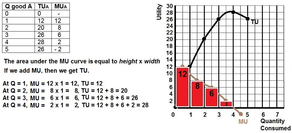
Utility is the reason we consume a good or
service. You might call it the satisfaction that we get when we
consume something. I get satisfaction (utility) when I drive my boat.
I get utility (satisfaction) when I go to the dentist.
"Marginal" means EXTRA or ADDITIONAL. So if I
drive my boat a second time I get some additional (marginal)
utility.
According to the law of diminishing marginal
utility, the EXTRA (not the total) utility diminishes for each
additional unit consumed. The first time I drive my boat in the
spring I really enjoy it. But after a few weekends of boating it
doesn't give me as much additional satisfaction as the first time. I
still go boating. My total utility still goes up. But the MARGINAL
(extra) utility I get from one more day goes down.
Back to the President Trump Example. Since we
start with no pants, the FIRST PAIR we get from President Trump gives
us A LOT of utility (satisfaction). But, since President Trump STILL
HAS BILLIONS of pairs of pants left, giving us 300 million causes his
utility (satisfaction) to go down only A LITTLE. Therefore, when we
went from NOT FAIR to MORE FAIR we gained more satisfaction than
Trump lost. Overall, a more fair distribution of pants caused
society's total utility (remember, "society" includes all of us AND
President Trump ) to increase.
The 5Es of Economics

Scarcity
and Exchange- EconMovies #1: Star Wars
[6:39 YouTube ACDC Leadership]
NOTE: These are REVIEW videos only. In order to
learn the material you must read the assigned textbook readings,
watch the assigned lecture videos, and do problems. See the
MICWEBAPP
or the LESSONS
link for these assignments.
Unit 1: Markets are Efficient, Except
. . . Intro to Microeconomics
Lesson 1c: Scarcity and Budget
Lines
So, do you agree that it is GOOD for the people
of Florida if, after a hurricane strikes, the price of plywood (or
other products) increases from $10 a sheet to $30 a sheet? Or, that
it was GOOD when the Coca-Cola company (or other companies) layed off
6000 workers as they did in the year 2000 assuming that they could
still produce the same quantity, but with fewer workers? Even if you
do not agree, do you understand that these things will reduce
scarcity and increase society's satisfaction? In lesson 5a we will
learn why the prices of products like gasoline, soda pop, and junk
food, may be TOO LOW. (Isn't this fun?)
Lesson 1c introduces our first graphic MODEL:
the budget line. For many students microeconomics is a difficult
course. I think there are two reasons for this. First, we will learn
theories or models, rather than facts. Facts are easy to memorize.
Theories or models have to be learned and practiced. And second, we
will express our theories or models on graphs, and many students do
not like graphs. If you want to be successful in this course you must
learn to use our graphical models. You must be able to draw the
graphs correctly from memory, you must understand what each line on
the graph represents, and you must know why each line has the shape
that it does. For each graph be able to: DEFINE, DRAW, DESCRIBE its
shape. Be sure to study the graphs in the textbook carefully and plot
all the graphs in the yellow pages. Finally, an easier way to view
graphs is to remember that each point on a graph represents two
numbers. Find a point on a graph, then find the two number from the
graph's axes.
Note: not all models are graphs. For example,
the 5Es of Economics is a model of the issues studied by
economists.
1c Something Interesting - Why are we
studying this?
|
USING MODELS: In this lesson we will learn our
first MODEL - the budget line. We will study many MODELS this semster
and most models will be represented by graphs. Why do economists use
so many models?
The paragraph below introduces a MOOC from the
University of Michigan called "Model Thinking". I was a bit surprised
that there is a whole couse just on using models, but it highlights
the importance of models in understanding the world around
us.
"We live in a complex world with
diverse people, firms, and governments whose behaviors aggregate
to produce novel, unexpected phenomena. We see political
uprisings, market crashes, and a never ending array of social
trends. How do we make sense of it? Models. Evidence
shows that people who think with models consistently outperform
those who don't. And, moreover people who think with lots of
models outperform people who use only one [emphasis
added]. Why do models make us better
thinkers? Models help us to better organize information - to make
sense of that fire hose or hairball of data (choose your metaphor)
available on the Internet. Models improve our abilities to make
accurate forecasts. They help us make better decisions and adopt
more effective strategies. They even can improve our ability to
design institutions and procedures. In this class, I present a
starter kit of models: I start with models of tipping points. I
move on to cover models explain the wisdom of crowds, models that
show why some countries are rich and some are poor, and models
that help unpack the strategic decisions of firm and politicians.
"
SOURCE: https://www.coursera.org/learn/model-thinking
OPTIONAL - More information about the
importance of using models:
Ch 1, pp. 4-11, (19th, 3-11), "The Economic
Perspective", "Theories, Principles, and Models", "Microeconomics and
Macroeconomics", "Individual's Economizing Problem"
Lecture
Outline
1c Assignments: Video
Lectures
|
WHAT IS ECONOMICS: SCARCITY, THE 5Es, AND MAKING
CHOICES
1.1.1 Scarcity
- Defining Economics 6:35
[MyNotes]
1.1.2
What
Economists Do 13:20
[
Summary] [Quiz]
[MyNotes]
1.1.3
Macroeconomics
and Microeconomics 11:21
[MyNotes]
EconMovies-
Episode 2: Monty Python and the Holy Grail - Marginal
Analysis (YouTube ACDCLeadership)
5:27
BUDGET
LINES
3.2.1 Constructing
a Consumer's Budget Constraint 9:36
[MyNotes]
3.2.2
Understanding
a Change in the Budget Constraint 5:02
[MyNotes]
1c Outcomes - What you should
learn
|
TOPICS
- Definition of economics
- Economic models (Why do economists use all
those graphs?)
- Budget lines
- Resources (Four Factors of Production)
OUTCOMES
- Define economics and describe the four
components of the definition:
- social science
- choice
- scarcity
- maximizing satisfaction
- What are economic models and why do
economists use them?
- Explain the importance of ceteris
paribus in formulating economic principles.
- Differentiate between microeconomics and
macroeconomics.
- Defne and draw budget lines. Explain what
happens to a budget line when income and prices
change.
- How does the budget line illustrate the
necessity of making choices?
- Define and give examples of the four types
of resources (factors of production) and know the payment for
each
Key Terms
Flash Cards - Click Here
Key Terms:
economics, economic model,
microeconomics, macroeconomics, utility, rational choice,
opportunity cost, benefit-cost analysis (marginal analysis),
ceteris paribus (other things equal assumption), budget line,
budget constraint, factors of production, resource, land, labor,
capital, entrepreneurial ability
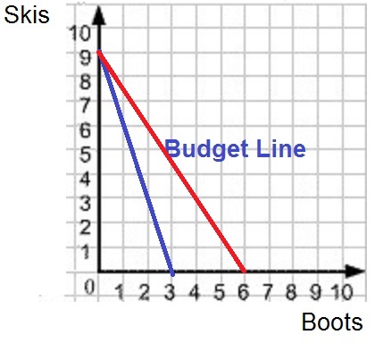
Budget
Lines
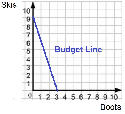
Assume the Price of X (Px) is $1 and the Price
of Y (Py) is $2 and you have $10 to spend. (income - $10).
1. Draw the budget line.
2. What happens to the budget line if your income decreases to
$6?
3. Assume your income is $10, and the Px is $1 and Py is $2. What
happens to the budget line if Py decreases to $1?
4. Assume your income is $10, and the Px is $1 and Py is $2. What
happens to the budget line if Px increases to $2?
Budget Line
Budget Line: Income
Increases
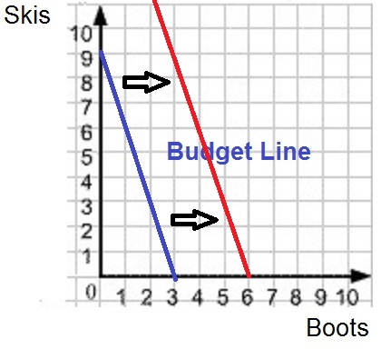
Budget Line: Price
Decreases
Scarcity
and Exchange- EconMovies #1: Star Wars
[6:39 YouTube ACDC Leadership]
NOTE: These are REVIEW videos only. In order to
learn the material you must read the assigned textbook readings,
watch the assigned lecture videos, and do problems. See the
MICWEBAPP
or the LESSONS
link for these assignments.
Unit 1: Markets are Efficient, Except
. . . Intro to Microeconomics
1d Making Choices: Production
Possibilities Curve (PPC) and Benefit Cost Analysis
(BCA)
Here we will study our second graphical model:
the Production Possibilities Curve (PPC), and we then will learn a
tool for making decisions that we will use throughout the course:
Benefit-Cost Analysis (BCA). Basically what we are doing is setting
the stage for making economic decisions. Remember: economics is the
social science concerned with how we CHOOSE to use our limited
resources to maximize society's unlimited wants, or, how we make
decisions.
The production possibilities curve will show us
that we must make choices and all choices have costs. Economists call
these "opportunity costs". ALL COSTS IN ECONOMICS ARE OPPORTUNITY
COSTS. Whenever we discuss the "costs" of doing something we will
mean the complete opportunity cost.
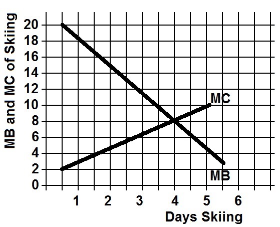
Benefit-cost analysis (BCA) is a model that
explains how to make the best decision possible. BCA means we should
select all options where the marginal benefits (MB) are greater than
the marginal costs (MC) -- up to where MB = MC. When the MB = MC then
we have made the best decision possible. NOTE: "marginal" means
"extra" or "additional". So to make the best decision possible select
all options where the extra benefits that you get from the decision
are greater than the extra costs of the decision. One more thing: to
make the best decisions we look only at MARGINAL costs and benefits
and we ignore FIXED, or SUNK, costs (i.e. ignore things that will not
change no matter what choice is made).
We will use BCA many times throughout this
course. In lesson 6a we will use BCA to decide how much to buy to
maximize our satisfaction. In lessons 8/9a, 8/9b, 10a, 10b, 11a, and
11b we will use it to decide how much to produce to maximize profits.
In lessons 12a and 13a we use BCA to decide how many to hire to
maximize profits.
Notice that economists look at EXTRA benefits
and EXTRA costs. We call this "thinking on the margin". Students are
used to thinking about TOTAL benefits and TOTAL costs. We do not want
total benefits to equal total costs, but we do want MB to equal MC.
You probably know that it is best if the total benefits are a lot
higher than total costs. What you will learn is that when MB = MC,
then the difference between total benefits and total costs will be
the greatest.
Be sure you understand Benefit-Cost Analysis
(BCA)!
What is the connection between the PPC and BCA?
Well, when studying the PPC you will learn the important concept of
"opportunity cost". Learn the definition well. Since all costs in
economics are opportunity costs, then when using BCA, "marginal
costs" mean the additional opportunity costs.
1d Something Interesting - Why are we
studying this?
|
The link below discusses a study that concludes
that drivers of cars with air bags have more accidents. Why would
airbags in cars cause more accidents (see the link below)?
After studying this lesson you should be able
to use Benefit-Cost Analysis (MB=MC) to answer this question. When
airbags were first put in cars how did that change the extra benefits
of driving fast (MB) and the extra costs of driving fast (MC)?
ANSWER: airbags reduce the extra costs of driving fast by making a
crash safer.
Drivers
with airbags may take more risks
A similar question for skiers is why did the
invention of avalanche airbags cause more people to become caught in
avalanches (see below)? After studying this lesson you should be
able to use Benefit-Cost Analysis (MB=MC) to answer this
question.
In a March
2013 blog post written by Utah
Avalanche Center Director Bruce Tremper . . . Tremper says airbags
are providing a false sense of security, leading more skiers into
high-consequence terrain, and thus decreasing the effectiveness of
said airbag.
"Each gizmo we buy to increase our
safety usually cause us to increase our level of risk at the
same time. For instance, when we added seat belts and airbags
to cars, yes fatalities decreased, but it also allowed us to
drive faster, farther, crazier and talk on our mobile phones at
the same time. So safety measures usually work but not nearly
as well as we would hope because people just increase their
risk (and “utility”) at the same time. In avalanche
airbag case, we will also get more powder, more fun, and more
risk in the bargain . . . . people will increase their exposure
to risk because of the perception of increased safety, which
will cancel out some, but not all, of the effectiveness of
avalanche airbag."
What are avalanche airbags?
https://www.youtube.com/watch?v=h7QFRXc0R8M
pp. 10-18, (19th, 11-20), "Society's
Economizing Problem", "Production Possibilities Model", "Optimal
Allocation" especially Fig 1.3, "The Economics of War" (box),
"Unemployment, Growth, and the Future"
pp. 6-7, (19th, 5), "Marginal Analysis:
Comparing Benefits and Costs"
Drivers
with airbags may take more risks
Lecture
Outline
1d Assignments: Video
Lectures
|
PRODUCTION POSSIBILITIES
1.4.1 Understanding
the Concept of Production Possibilities
Frontiers 24:46
[MyNotes]
1.4.2
Understanding
How a Change in Technology Affects the PPF
10:10 [MyNotes]
ECONMOVIES
Episode 3: Monsters Inc. and the Production Possibilities
Curve
MAKING
CHOICES: THE ECONOMIC WAY OF THINKING -- BENEFIT-COST ANALYSIS (also
called Marginal Analysis or Cost-Benefit Analysis)
EconMovies-
Episode 2: Monty Python and the Holy Grail - Marginal
Analysis (YouTube ACDCLeadership
5:27)
Thinking
at the Margin (YouTube LearnLiberty
4:32)
Incentives
and Marginal Analysis (YouTube
MrHurdleHistory 8:54)
CIRCULAR
FLOW MODEL
Micro
1.1 The BIG Picture- AP Economics Overview (with links to
playlists) (YouTube ACDCLeadership
12:49)
10.1.2 The
Circular Flow Model 9:38
[MyNotes]
1d Outcomes - What you should
learn
|
TOPICS
- Society's Economizing Problem: Production
Possibilities
- How to Make Choices: Benefit-Cost
Analysis
OUTCOMES
Production Possibilities
- Construct a production possibilities curve
(PPC) when given appropriate data; what is the production
possibilities curve (PPC) or production possibilities frontier
(PPF)?; what does it show?
- What are the assumptions behind the
PPC?
- Illustrate the following using the
production possibilities curve:
- - we must make choices
- choices have opportunity costs
- the law of increasing costs
- the effect of unemployment
- the effect of productive inefficiency
- the effect of economic growth
- how present choices affect future possibilities
- the effect of international trade
- it does NOT show the optimum product mix (allocative
efficiency)
- Explain WHY the PPC has the shape that it
does -- concave to the origin. What is the law of increasing cost?
Why are there increasing costs? (Draw, Define. Describe all
graphs)
- What would the PPC look like if there were
constant costs?
- What does a point outside the PPC
represent?
- What two things (2 Es) would a point inside
the PPC indicate?
- Summarize the general relationship between
investment and economic growth.
- Describe the two types of economic growth
("achieving the potential" and "increasing the potential") and
explain how are they shown on a PPC?
- What would cause a PPC to shift
inward?
- Use a PPC to illustrate the effect of
international trade
Benefit Cost Analysis
- define benefit cost analysis (BCA) and use
it to solve problems
- define "marginal" and give
examples
- define marginal benefits (MB) and marginal
costs (MC)
- know what happens if MC increase?
decrease?
- know what happens if MB increase?
decrease?
- draw MB and MC on a graph and explain their
shapes
- be able to find the optimum choice from a
table of total costs and total benefits and from a table of
marginal costs and marginal benefits
- use BCA to explain why Drivers
with airbags may take more risks or
why skiers
with air bags may take more risks
- what is a "sunk cost" (or fixed cost) and
why are they ignored when using benefit-cost analysis?
- explain why we ignore fixed, or sunk, costs
("Don't cry over spilt milk."). If you are deciding whether or not
to come to class today, why does it not matter that you have
already paid tuition? Why is the fact that you have paid tuition
irrelevant when trying to decide whether to attend class today or
skip?
Key Terms
Flash Cards - Click Here
Key Terms:
PPC:
production possibilities, necessity of choice, law of increasing
costs, concave to the origin, opportunity cost, constant cost,
benefit-cost analysis (marginal analysis), economic growth,
consumer goods, capital goods, shrinking PPC, nonproportional
growth
BCA:
marginal costs (MC), marginal benefits (MB), MB=MC Rule, sunk
(fixed) costs
Production
Possibilities Curve (PPC) - Click Here
Using
Benefit Cost Analysis (BCA) - Click Here
Click
here to see PPC questions
Using Benefit Cost Analysis (BCA)
Question:
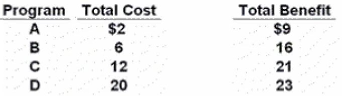
Use the above information on four different
highway programs of increasing scope to decide which program the
government should do.
All numbers are in billions of dollars.
Use Benefit Cost Analysis to answer the
question.
1d Key Graphs
|
|
The Production Possibilities
Curve (PPC)
PPC: Unemployment to Full
Employment and
Productive Inefficiency to Efficient (Achieving the
Potential)
PPC and Economic Growth
(Increasing the Potential)
Benefit Cost
Analysis
|
- Production
Possibilities Curve- Econ 1.1
[3:56 YouTube ACDC Leadership]
- Shifting
the Production Possibilities Curve (PPC)- Econ
1.2
[5:35 YouTube ACDC Leadership]
NOTE: These are REVIEW videos only. In order to
learn the material you must read the assigned textbook readings,
watch the assigned lecture videos, and do problems. See the
MICWEBAPP
or the LESSONS
link for these assignments.
Unit 1: Markets are Efficient, Except
. . . Intro to Microeconomics
Lesson 2a: Market Economies and
Trade
One reason why I use our textbook is because
they have a chapter on market economies and they used to have a
chapter on command economies (now just a small section). In this
lesson we find out for the first time that competitive market
economies are efficient, both allocatively and productively. This is
the result of the "invisible hand" of capitalism. This is a general
theme for the whole course that we will discuss again in lessons 3,
5, and lessons 8 to13. Many textbooks simply assume that students
know what a capitalist economy (market economy) is because we live in
one here in the United States. But, I learned long ago that students
do not understand the characteristics of captialism nor the benefits
of, or the problems with, market economies. All over the world
countries are moving away from command economies toward a market
economy. Why? We will learn it is because market economies are better
at achieving allocative and productive efficiency, and economic
growth, but they do seem have a problem with equity and at times full
employment.
One characteristic of a market economy is a
limited role for government. Periodically we will discuss just WHAT
IS the economic role of government? What should the government do, or
not do? This is where Republicans and Democrats seem to have a
fundamental disagreement, but I think they agree more than they
believe. Remember this: the economic goal of society is to maximize
its satisfaction (reduce scarcity as much as possible). And they do
this by achieving the 5Es. The economic role of government then ALSO
should be to achieve the 5Es. We will return to this issue of the
economic role of government at different times thoughout the
course.
Our first discussion of this economic role for
government will be FREE TRADE. Should the United States have free
trade with other countries like Mexico and China, or should the
government impose trade restrictions? We will examine this question
by using the production possibilities model that we learned in lesson
1d.
2a Something Interesting - Why are we
studying this?
|
The Gains from Trade:
Read the first four paragraphs of
The
Mystical Power of Free Trade.
After studying this lesson you should
understand:
- why "society benefits from
allowing its citizens to buy what they wish--even from
foreigners." (i.e. free trade helps society),
- and why "people resist this conclusion,
sometimes violently"
pp. 31-51 (19th ed. Ch. 2 ALL), "The Market
System and Circular Flow"
pp. 534-542, (19th, 474-482), "The Economic
Basis for Trade"
A
Comparison of Market Economics and Command Economies
Lecture
Outline
2a Assignments: Video
Lectures
|
ECONOMIC SYSTEMS
1.1.4 An
Overview of Economic Systems 10:50
[MyNotes]
Power
of the Market (YouTube LibertyPen)
1:14 [MyNotes]
17.5.3
Comparative
Economic Performance 12:16
[MyNotes]
OPTIONAL:
Paul
Solman Video: Capitalism vs. Socialism - The Cuban
Quandary (YouTube PBS NewsHour)
13:56
SPECIALIZATION
AND GAINS FROM TRADE
1.5.1 Defining
Comparative Advantage with the Production Possibilities
Frontier 22:10 [MyNotes]
1.5.2 Understanding
Why Specialization Increases Total Output
6:46 [MyNotes]
1.5.3 Analyzing
International Trade Using Comparative
Advantage 25:35
[MyNotes]
KEY PROBLEM: The
gains from trade
2a Outcomes - What you should
learn
|
TOPICS
- How Countries Make Economic Choices:
Economic Systems
- Market Economies
- Command Economies
- Capitalism and the Five Fundamental
Questions
- Capitalism and Efficiency (the invisible
hand)
- The Gains from Trade
OUTCOMES
Economic Systems
- Laissez-faire economic system
- Centrally Planned Economy
- Mixed economic systems
- The Bolshevik Revolution
- Contributing factors to the collapse of the
Soviet Union
- characteristics of the market
system
- the important role of profits and
losses
- property rights
- the "invisible hand" of
capitalism
- the coordination problem
- the incentive problem
- be able to draw and explain the Circular
Flow Model
- Why are market economies more efficient
than command economies both allocatively and
productively?
- What is the "invisible hand" of
capitalism?
- How does trade increase productive
efficiency and therefore output?
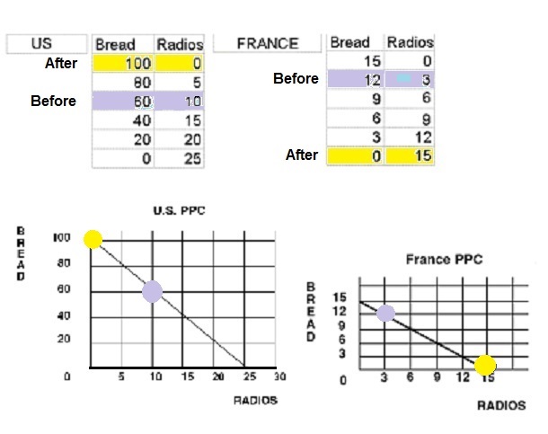
Gains From Trade
- calculate how specialization and trade
increases output using the production possiblilities tables and
graphs of two different countries
- straight line PPCs (constant
costs)
- absolute advantage
- comparative advantage
- calculate comparative
advantage
- specialization and trade
- calculate the gains from specialization
and trade
Key Terms
Flash Cards - Click Here
Key Terms:
economic system, command system (centrally
planned, socialism), market system (capitalism, laissez-faire), mixed
economic system, Bolshevik revolution, self interest, private
property, freedom of enterprise and choice, competition, market,
specialization, consumer sovereignty, dollar votes, invisible hand,
creative destruction, coordination problem, incentive problem,
circular flow diagram, product market, resource market, opportunity
cost, absolute advantage, comparative advantage, gains from trade,
free trade.
The
Gains from Trade - Click Here
Click on the link above to learn how to do this
problem.
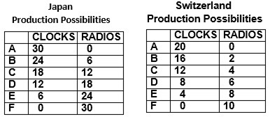
Assume that prior to specialization and trade,
Japan produced at point D and Switzerland produced at point E.
Calculate the possible gains from specialization and
trade.
Comparative Advantage and the Gains from
Trade
Circular Flow Model of
Capitalism
Market
Economy (Capitalism)
The
Gains from Trade
- Econ
1.6- Economic Systems: Why is Communist China doing so
well?
[4:13 YouTube ACDC
Leadership]
- Comparative
advantage specialization and gains from trade | Microeconomics | Khan
Academy
[8:55 YouTube Khan Academy]
NOTE: These are REVIEW videos only. In order to
learn the material you must read the assigned textbook readings,
watch the assigned lecture videos, and do problems. See the
MICWEBAPP
or the LESSONS
link for these assignments.
Unit 1: Markets are Efficient, Except
. . . Intro to Microeconomics
Lesson 3a: Demand
If the price of pizza goes up, what happens to
the demand for pizza? . . . . . . . . . . . . . . . . . . . NOTHING!
Nothing happens to the demand for pizza if the price
changes!
The next three lessons introduce the demand and
supply model for explaining how prices arise and change in a market
economy. Learn these lessons well. Do the assigned problems. Draw the
graphs in the yellow pages and while you are reading and studying.
DRAW GRAPHS! Get used to using the graphs to help you answer
questions. If you are avoiding drawing the graphs you will do poorly
and not get the practice that you need to learn the concept. Be sure
to LABEL the axes of every graph that you draw.
So why doesn't the demand for pizza change if
the price changes? Because economists have a different definition of
"demand". Demand is NOT the quantity that we buy. If the price of
pizza goes up we will buy less, but that is not what "demand" means
in economics. Economists tend to be precise with their definitions
and sometimes their definitions are different than the more commonly
used definitions. Things like "scarcity", "investment", "cost",
"demand", and "supply", have different definitions in economics than
what you may already know. Learn our definitions! Demand is not how
much we buy. Demand has a different definition in economics. "Demand"
means the "demand graph".
Remember, that econmists use models (like the
supply and demand model) to simplify the real world. They do this by
isolating certain variables from all the clutter found in reality.
Then by changing one variable at a time economists can see what
effect it will have. In this lesson we will learn the economic
definition of DEMAND and plot the demand graph. Then, we will look at
one variable at a time to see what effect they have on the demand
curve. We call these variables the "non-price determinants of
demand". They are: Pe, Pog, I, Npot, T (P,P,I,N,T). LEARN THEM! LEARN
THEM WELL! Know how each one affects the demand curve. Be sure to do
the yellow pages.
3a Something Interesting - Why are we
studying this?
|
What is that Campbell's Pork and Beans can doing
on the display for VanCamp's Pork and Beans (see below)?

After studying this lesson you will be able to
draw a graph illustrating what happened to the demand for
Campbell's Pork and Beans when a customer took a can out of their
shopping cart and placed it on this display of VanCamp's Pork and
Beans that were on sale.
What happend to the demand for Campbell's and
which non-price determinant of demand explains why that Campbell's
soup can is there?
ANSWER: The demand for Campbell's decreased
because the price of a substitute good, VanCamp's, decreased. There
has been no change in the demand for VanCamp's.
pp. 53-59, (19th, 47-53), "Markets",
"Demand"
Optional,
but very useful
Lecture
Outline
3a Assignments: Video
Lectures
|
2.1.1 Understanding
the Determinants of Demand 11:58
[MyNotes]
2.1.2
Understanding
the Basics of Demand 11:54
[MyNotes]
2.1.3
Analyzing
Shifts in the Demand Curve 8:13
[MyNotes]
2.1.4
Changing
Other Demand Variables 10:43
[MyNotes]
2.1.5
Deriving
a Market Demand Curve 9:16
[MyNotes]
OPTIONAL
Snow Day Lecture - During the 2018-2019 school year we had a snow day
when lesson 3a was scheduled in our on-campus class. To avoid losing
a day of class I recorded the lesson 3a lecture and posted it online.
Here it is: Lesson
3a Snow Day lecture (1hour 15
minutes)
OPTIONAL:
The
Law of Demand (econclassroom.com
11:24)
Changes
in Demand versus Changes in Quantity
Demanded (econclassroom.com
5:52)
The
Determinants of Demand
(econclassroom.com 11:07)
3a Outcomes - What you should
learn
|
TOPICS
- Definition of demand
- Changes in Demand vs. Changes in Quantity
Demanded
- Non-price determinants of demand and how
they affect the demand curve
OUTCOMES
- define demand (note: it has a
DIFFERENT DEFINITION in economics)
- If the price of pizza goes up, why does the
demand for pizza stay the same?
- be able to correctly draw and label a
demand graph
- why do economists employ the ceteris
paribus assumption when creating a demand curve?
- what is the law of demand?
- why is the demand curve downward sloping
(three explanations)
- list the non-price determinants of demand
(Pe. Pog, I, Npot, T) or (P, P, I, N, T ) and understand how they
affect the demand schedule and curve. This is VERY IMPORTANT. BE
ABLE TO DO THIS! See the 3a/3b/3c yellow pages.
- explain the difference between the a
"change in the quantity demanded" and a "change in
demand"
- what is an "increase in demand" and a
"decrease in demand" and show how they affect the demand schedule
and the demand curve
- what is "market demand"?
- what is that Campbell's Pork and Beans can
doing on the display for VanCamp's Pork and Beans (see picture at
left)? Which non-price determinant of demand explains why that
Campbell's soup can is there? Draw a supply and demand graph
illustrating what happened in the market for Campbell's Pork and
Beans when VanCamp's were put on sale.
3a Non-Price Determinants of Demand
and Supply
|
Non-Price Determinants of Demand (PPINT)
Pe -- expected price
Pog -- price of other goods
1) substitute goods
2) complementary goods
3) independent goods
I -- income
1) normal goods
2) inferior goods
N -- number of POTENTIAL consumers
T -- tastes and preferences
Non-Price Determinants of Supply
(PPPTTN)
Pe -- expected price
Pog -- price of other goods produced by same firm
Pres -- price of resources
T --technology
T --taxes and subsidies
N -- number of producers/sellers
NON-PRICE DETERMINANTS OF DEMAND
Pe -- expected price
 Pe
in the future
Pe
in the future  D today
 Pe in the future
D today
Pe in the future
D today
Pog -- price of other goods
1) substitute goods
P Maxwell House coffee
D Folgers coffee
P of one product
D of its substitute
2) complementary goods
P of wieners
D of buns
P of one product
D of its compliment
I -- income
1) normal goods
Income
D for normal goods
Income
D for normal goods
2) inferior goods
Income
D for inferior goods
Income
D for inferior goods
Npot -- number of POTENTIAL
consumers
Npot
D
Npot
D
T -- tastes and preferences
Tastes for a product
D for that product
Tastes for a product
D for that product
NON-PRICE DETERMINANTS OF SUPPLY
Pe -- expected price
Pe in the future
S today
Pe in the future
S today
Pog -- price of other goods also produced by
the same firm
P soybeans
S corn
P soybeans
S corn
Pres -- price of resources
worker's wages
cost of making cars
S cars
Pres
costs
S
Pres
costs
S
Tech --technology
Improved technology
costs
S
Tax --taxes and subsidies
Taxes
costs
S
Taxes
costs
S
Subsidies
costs
S
Subsidies
costs
S
N -- number of
producers/sellers
Nproducers
S
Nproducers
S
Key Terms
Flash Cards - Click Here
Key Terms:
demand, quantity demanded, law of
demand, market demand, horizontal summation, income effect,
substitution effect, diminishing marginal utility, change in
demand, change in quantity demanded, increase in demand, decrease
in demand, non-price determinants of demand, normal good, inferior
good, substitute good, complementary good (complement),
independent goods
The Demand Curve
Changes in Demand
Increase in Demand
Decrease in Demand
Market Demand (horizontal
summation of individual demand curves)
- Demand
and Supply Explained- Econ 2.1
[6:20 YouTube ACDC Leadership]
NOTE: These are REVIEW videos only. In order to
learn the material you must read the assigned textbook readings,
watch the assigned lecture videos, and do problems. See the
MICWEBAPP
or the LESSONS
link for these assignments. .
Unit 1: Markets are Efficient, Except
. . . Intro to Microeconomics
Lesson 3b: Supply
If the price of pizza goes up what happens to the
SUPPLY of pizza? . . . . . . . . . . NOTHING!
A change in the price of a product does not
affect its supply, or its demand. When the price goes up the QUANTITY
SUPPLIED will increase, but the supply does not change. Learn the
difference between "supply" and "quantity supplied". "Supply" does
NOT MEAN the quantity available for sale. Supply has a different
definition in economics. "Supply" means the "Supply
graph".
So what would cause the supply graph, or supply
itself, to change? Those things that cause supply to change are
called the "non-price determinants of supply". They are: Pe, Pog,
Pres, Tech, Tax, Nprod (P,P,P,T,T,N). See the Yellow
Pages.
Remember, the goal of lessons 3a, 3b, and 3c is
to learn a model that will help us understand why prices are what
they are and why prices change. In the next lesson we will put demand
and supply together and use the model (graph) to find the prices of
products. Then, and more importantly, we will see what causes prices
to change. If you hear on the news, or read in your news app, that
the price of gasoline is going down, we will be able to explain WHY.
The causes of changes in prices of products are the five non-price
determinants of demand (Pe, Pog, I, Npot, T) and/or the six non-price
determinants of supply (Pe, Pog, Pres, Tech, Tax, Nprod.). Whenever
you hear that the price of something is changing think of these 11
possible causes.
3b Something Interesting - Why are we
studying this?
|
Read the short news article below on the
declining price of gasoline (Dec. 2015). Paragraph 10 states
"Plunging oil prices are the main factor driving down the price at
the pump."
Gas
falls below $2 a gallon [http://money.cnn.com/2015/12/20/news/economy/aaa-2-dollar-gas/index.html]
After studying this lesson you should be able
to:
(1) list the non-price determinants of
supply
(2) select the determinant that is the cause of the decline in
gasoline prices discussed in the news article, and
(3) graph the effect that the change in the determinant will have on
the supply curve for gasoline.
pp. 59-62, (19th, 53-56), "Supply"
http://www.npr.org/blogs/parallels/2015/01/28/382173205/where-is-all-that-excess-oil-going
[Why are they storing oil? What is happening to supply? Which
determinant has caused the supply to change?]
Optional,
but very useful
Lecture
Outline
3b Assignments: Video
Lectures
|
2.2.1 Understanding
the Determinants of Supply 7:25
[MyNotes]
2.2.2
Deriving
a Supply Curve 9:49
[MyNotes]
2.2.3
Understanding
a Change in Supply versus a Change in Quantity
Supplied 6:52 [MyNotes]
2.2.4
Analyzing
Changes in Other Supply Variables 8:47
[MyNotes]
2.2.5 Deriving
a Market Supply Curve from Individual Supply
Curves 7:16 [MyNotes]
3b Outcomes - What you should
learn
|
TOPICS
- Definition of supply
- Changes in Supply vs. Changes in Quantity
Supplied
- Non-price determinants of supply and how
they affect the supply curve
OUTCOMES
- define supply (note: it has a DIFFERENT
DEFINITION in economics)
- be able to correctly draw and label a
supply graph
- if the price of pizza goes up why does the
supply not change?
- why do economists employ the ceteris
paribus assumption when creating a supply curve?
- what is the law of supply?
- why is the supply curve upward sloping (two
explanations)
- list the non-price determinants of supply
(Pe, Pog, Pres, Tech, Taxes, Nprod) or (P,P,P,T,T,N) and
understand how they affect the supply schedule and curve. This is
VERY IMPORTANT. BE ABLE TO DO THIS! See the 3a/3b/3c yellow
pages.
- explain the difference between the a
"change in the quantity supplied" and a "change in
supply"
- what is an increase in supply and a
decrease in supply and show how they affect the supply schedule
and the supply curve
- what is "market supply"?
- Read the following and answer these
questions:
- Which determinant has
changed?
- Will it affect S or D of
gasoline?
- Will the S or D of gasoline increase or
decrease? Shift to the right or to the left?
"According to the Lundberg Survey, the
average price for regular gasoline dropped 3.99 cents over the
three weeks up to July 11 to $3.6699 per gallon. . . . Lundberg
explained that the average gasoline price continues to decrease
because refiners, enjoying the lower crude oil prices in the
market, are passing down the savings to the consumers.
"
From: http://www.techtimes.com/articles/10378/20140714/average-price-of-gasoline-in-u-s-drops-four-cents-now-at-3-67-a-gallon.htm
3b Non-Price Determinants of Demand
and Supply
|
Non-Price Determinants of Demand (PPINT)
Pe -- expected price
Pog -- price of other goods
1) substitute goods
2) complementary goods
3) independent goods
I -- income
1) normal goods
2) inferior goods
N -- number of POTENTIAL consumers
T -- tastes and preferences
Non-Price Determinants of Supply
(PPPTTN)
Pe -- expected price
Pog -- price of other goods produced by same firm
Pres -- price of resources
T --technology
T --taxes and subsidies
N -- number of producers/sellers
NON-PRICE DETERMINANTS OF DEMAND
Pe -- expected price
Pe
in the future
D today
Pe in the future
D today
Pog -- price of other goods
1) substitute goods
P Maxwell House coffee
D Folgers coffee
P of one product
D of its substitute
2) complementary goods
P of wieners
D of buns
P of one product
D of its compliment
I -- income
1) normal goods
Income
D for normal goods
Income
D for normal goods
2) inferior goods
Income
D for inferior goods
Income
D for inferior goods
Npot -- number of POTENTIAL
consumers
Npot
D
Npot
D
T -- tastes and preferences
Tastes for a product
D for that product
Tastes for a product
D for that product
NON-PRICE DETERMINANTS OF SUPPLY
Pe -- expected price
Pe in the future
S today
Pe in the future
S today
Pog -- price of other goods also produced by
the same firm
P soybeans
S corn
P soybeans
S corn
Pres -- price of resources
worker's wages
cost of making cars
S cars
Pres
costs
S
Pres
costs
S
Tech --technology
Improved technology
costs
S
Tax --taxes and subsidies
Taxes
costs
S
Taxes
costs
S
Subsidies
costs
S
Subsidies
costs
S
N -- number of
producers/sellers
Nproducers
S
Nproducers
S
Key Terms
Flash Cards - Click Here
Key Terms:
supply, quantity supplied, market
supply, law of supply, change in supply, change in quantity
supplied, increase in supply, decrease in supply, non-price
determinants of supply
The Supply Curve
Changes in Supply
Increase in Supply
Decrease in Supply
- Demand
and Supply Explained (2 of 2) - Econ 2.2
[4:54 YouTube ACDC Leadership]
NOTE: These are REVIEW videos only. In order to
learn the material you must read the assigned textbook readings,
watch the assigned lecture videos, and do problems. See the
MICWEBAPP
or the LESSONS
link for these assignments.
Unit 1: Markets are Efficient, Except
. . . Intro to Microeconomics
Lesson 3c: Market Equilibrium and
Efficiency
We are going to learn two very important things
in this lesson: How to find WHAT WE GET and WHAT WE WANT.
First, we will put demand and supply together
and learn how to use the model to to see how much businesses will
produce to maximize their profits (WHAT WE GET) and why products have
the prices that they do. We will learn how to use the model to see
what causes prices to change.
If you hear on the news or read in your news
app, that the price of gasoline is going down, we will be able to
explain WHY. The causes of changes in prices of products are the five
non-price determinants of demand (Pe, Pog, I, Npot, T) and/or the six
non-price determinants of supply (Pe, Pog, Pres, Tech, Tax, Nprod.).
Whenever you hear that the price of something is changing think of
which of these 11 possible causes have changed, draw the graph and
shift the appropriate demand and/or supply graph, and the graph will
show the price changing.
Second, after we learn that in a competitive
market economy the interaction of demand and supply will determine
what the prices of products will be and how much people will buy at
that price, we will ask: Is this the allocatively efficient quantity
and price (WHAT WE WANT)? Our goal is to show that in a competitive
market prices and quantities will change until allocative efficiency
is achieved.
In lesson 2a we learned that competitive
markets are allocatively efficient. This means they will produce the
quantity of goods that maximizes the society's satisfaction. After
studying lessons 3a, 3b, and 3c we will be able to show the
allocatively efficient price and quantity on a graph. We will learn
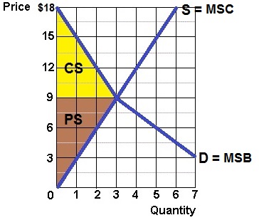
two of the three ways to find the allocatively efficient quantity:
(1) quantity were MSB = MSC, and (2) the quantity where consumer
surplus plus producer surplus is maximized. In Unit 3 we will learn a
third way to find the allocatively efficient quantity" the quantity
where P = MC (price equals marginal cost).
Competitive markets are efficient.
3c Something Interesting - Why are we
studying this?
|
Read the first few paragraphs of Hybrid
Car Prices Increasing Due To High Gas Prices.
In lesson 3a you learned how the non-price
determinants of demand (Pe, Pog, I, N, T) affect the demand curve.
In lesson 3b you learned how the non-price
determinants of supply (Pe, Pog, Pres, Tech, Tax, Nprod) affect the
supply curve.
After studying this lesson you will be able to
use these determinants and the supply and demand graphs to explain
why prices change.
For example you will understand why: "It's
becoming almost an annual tradition: As fuel prices rise in the
spring, so do the prices of hybrid cars. "
pp. 62-67, (19th, 56-61), "Market Equilibrium",
"Changes in Supply, Demand, and Equilibrium"
pp. 75-80, (19th, 69-74 ), "Additional Examples
of Supply and Demand"
pp. 85-90, (19th, 93-99), "Efficiently
Functioning Markets "
Supply,
Demand, and Economic Efficiency
Optional,
but very useful
Lecture
Outline
3c Assignments: Video
Lectures
|
PUTTING SUPPLY AND DEMAND TOGETHER
2.3.1 Determining
a Competitive Equilibrium 11:04
[MyNotes]
2.3.2 Defining
Comparative Statics 7:02
[MyNotes]
2.3.3
Classifying
Comparative Statics 11:54
[MyNotes]
AC
Micro
2.4 Double Shifts in Supply and Demand: Econ Concepts in 60
Seconds (2:34)
EconMovies:
Episode
4: Indiana Jones (Demand, Supply, Equilibrium,
Shifts) (7:02)
MARKETS AND
EFFICIENCY
Consumer
and Producer Surplus in the Linear Demand and Supply
Model (econclassroom.com
10:01)
Efficiency
and Equilibrium in Competitive Markets
(econclassroom.com 11:48)
3c Outcomes - What you should
learn
|
TOPICS
- Market Equilibrium
- Market Equilibrium and Changes in D and
S
- Market Equilibrium and Allocative
Efficiency
- MSB=MSC
- maximum consumer plus producer
surplus
OUTCOMES
Equilibrium
- what are the two assumptions of a
competitive equilibrium?
- there are many buyers and sellers in the
market
- who have no influence over the price;
i.e. they are price takers
- define equilibrium; define market
equilibrium
- what happens if the price is below the
equilibrium price? If it is above it?
- how to find the equilibrium price and
quantity on a supply and demand schedule and graph
- define "shortage" and "surplus" and explain
using a supply and demand graph
- what is the "bidding
mechanism"?
- the three (or four) steps to finding a new
equilibrium when a non-price determinant changes and how to use
them
- what happens to the equilibrium price and
quantity if (1) demand increases, (2) demand decreases, (3) supply
increases, and (4) supply decreases.
- what happens if both supply and demand
change
Markets and Efficiency
- be able to use two models to show why
competitive market economies achieve allocative efficiency
- MSB=MSC
- maximum consumer plus producer
surplus
- define marginal social benefit and explain
why it is often measured by the demand curve
- define marginal social cost and explain why
it is often measured by the supply curve
- explain why allocative inefficiency occurs
where MSB > MSC causing an underallocation of resources (too
little produced); show on graph using the MSB=MSC
model
- explain why allocative inefficiency occurs
where MSB < MSC causing an overallocation of resources (too
much produced); show on graph using the MSB=MSC model
- be able to find WHAT WE GET and WHAT WE
WANT on the MSB=MSC model graph
- define consumer surplus and producer
surplus and shade them in on a supply and demand graph
- define deadweight loss and be able to
locate it on a supply and demand graph if too much or too little
is produced
3c Non-Price Determinants of Demand
and Supply
|
Non-Price Determinants of Demand (PPINT)
Pe -- expected price
Pog -- price of other goods
1) substitute goods
2) complementary goods
3) independent goods
I -- income
1) normal goods
2) inferior goods
N -- number of POTENTIAL consumers
T -- tastes and preferences
Non-Price Determinants of Supply
(PPPTTN)
Pe -- expected price
Pog -- price of other goods produced by same firm
Pres -- price of resources
T --technology
T --taxes and subsidies
N -- number of producers/sellers
NON-PRICE DETERMINANTS OF DEMAND
Pe -- expected price
Pe
in the future
D today
Pe in the future
D today
Pog -- price of other goods
1) substitute goods
P Maxwell House coffee
D Folgers coffee
P of one product
D of its substitute
2) complementary goods
P of wieners
D of buns
P of one product
D of its compliment
I -- income
1) normal goods
Income
D for normal goods
Income
D for normal goods
2) inferior goods
Income
D for inferior goods
Income
D for inferior goods
Npot -- number of POTENTIAL
consumers
Npot
D
Npot
D
T -- tastes and preferences
Tastes for a product
D for that product
Tastes for a product
D for that product
NON-PRICE DETERMINANTS OF SUPPLY
Pe -- expected price
Pe in the future
S today
Pe in the future
S today
Pog -- price of other goods also produced by
the same firm
P soybeans
S corn
P soybeans
S corn
Pres -- price of resources
worker's wages
cost of making cars
S cars
Pres
costs
S
Pres
costs
S
Tech --technology
Improved technology
costs
S
Tax --taxes and subsidies
Taxes
costs
S
Taxes
costs
S
Subsidies
costs
S
Subsidies
costs
S
N -- number of
producers/sellers
Nproducers
S
Nproducers
S
Key Terms
Flashcards - Click Here
Market Equilibrium
equilibrium, market equilibrium,
bidding mechanism, surplus, shortage, scalping,
Efficiency
productive efficiency, allocative efficiency,
marginal social benefits, marginal social costs, "what we get", "what
we want", profit maximizing quantity, underallocation of resources,
overallocation of resources, consumer surplus, producer surplus,
deadweight loss
Beef
and Chicken
Almonds
McDonald's
Click on the links above to learn how to use a
supply and demand graph to show why prices and quantities change. The
exam 1 extra credit question will be similar to these problems.
Use the four-step process to explain what
happens to PRICE (P) and QUANTITY (Q) of the following goods using
the information provided in the short news articles below.
Four Step Process
1. Which determinant has
changed?
2. Will it affect Supply (S) or Demand (D)?
3. Will S or D increase or decrease?
4. GRAPH IT and show what happens to P and Q.
Non--Price Determinants of Demand
(PPINT)
Pe -- expected price
Pog -- price of other goods (subs and Complw)
I - income (normal and inferior goods)
N -- number of POTENTIAL consumers
T -- tastes and preferences
Non-Price Determinants of Supply
(PPPTTN)
Pe -- expected price
Pog -- price of other goods PRODUCED. BY THE SAME FIRM
Pres -- price of resources
T - technology of production
T -- taxes and subsidies
N -- number of sellers
Product: Beef. What happens to
P and Q? Circle and label determinants. Show effects on a
graph.
http://www.bloomberg.com/news/articles/2014-11-18/us-beef-supply-will-fall-again-in-2015-chicken-demand-will-rise
Domestic beef production has been
waning [decreasing] for years because of rising feed
and energy prices. A drought in 2012 caused feed prices to
spike and, in response, farmers thinned their herds.
Product: Chicken. What happens
to P and Q? Circle and label determinants. Show effects on a
graph.
http://www.bloomberg.com/news/articles/2014-11-18/us-beef-supply-will-fall-again-in-2015-chicken-demand-will-rise
It's been an expensive year to eat
beef, and 2015 doesn't look any cheaper. . . . Consumers have
traded down to less expensive meats such as chicken.
Product: Almonds. What happens
to P and Q? Circle and label determinants. Show effects on a
graph.
http://www.cnbc.com/2016/08/29/california-almond-harvest-may-break-records-despite-drought.html
With the drought easing in parts of
California, this year's almond harvest is shaping up to be a
record haul …. Consumers have already taken an interest in
almond products because of their "heart health"
benefits.
Product: McDonald's meals.
What happens to P and Q? Circle and label determinants. Show
effects on a graph.
http://www.bloomberg.com/news/articles/2014-10-20/mcdonald-s-costly-burgers-send-diners-to-fancier-rivals
Mike Hiner used to take his
grandsons to McDonald's when they wanted a treat. With higher
wage and food costs pushing up prices at the Golden Arches,
he's increasingly taking them to IHOP, Denny's and Chili's
instead . . . . The chain's diminishing appeal among budget
diners -- coupled with rising meat costs -- are projected to
take a bite out of third-quarter earnings due to be reported
tomorrow.
Market Equilibrium
Changes in Demand and Supply and the
Effects on Equilibrium P and Q
Market Equilibrium is
Efficient
MSB = MSC Model
Maximum Consumer + Producer Surplus
Model
- Shifting
Demand and Supply- Econ 2.3
[4:49 YouTube ACDC Leadership]
- Double
Shifts- Econ 2.5 (Technical Tuesday)
[3:26 YouTube ACDC Leadership]
- Micro
4.13 Dead Weight Loss- Key Graphs of
Microeconomics
[4:45 YouTube ACDC Leadership]
- Micro
2.7 Consumer and Producer Surplus and Dead Weight
Loss
[3:42 YouTube ACDC Leadership]
NOTE: These are REVIEW videos only. In order to
learn the material you must read the assigned textbook readings,
watch the assigned lecture videos, and do problems. See the
MICWEBAPP
or the LESSONS
link for these assignments.
Unit 1: Markets are Efficient, Except
. . . Intro to Microeconomics
Lesson 5a: Government Interference in
Markets and Market Failures (Negative
Externalities)
In lesson 3c we learned that competitive markets
are efficient and we learned two models to show that markets are
efficient: (1) MSB = MSC, and (2) maximum consumer plus producer
surplus. You must understand these models to understand lessons 5a
and 5b. In these lessons we learn that SOMETIMES markets are NOT
efficient.
When are product markets not
efficient?
1. when there is not competition
(monopolies and oligopolies - lessons 10a, 10b, 11a, and 11b)
2. when the government sets the price (price ceilings and price
floors - lesson 5a)
3. when the supply curve does not include all
of the costs of producing or consuming the product (negative
externalities - lesson 5a)
4. when the demand curve does not include all of the benefits of
consumption (positive externalities - lesson 5b)
5. when the products are "public goods" (lesson 5b).
6. when there is a Tragedy of the Commons (lesson 5b)
In this lesson we also will begin our look at
the role of the government in a market economy. This would be a good
time to review lesson 2a. In lesson 2a we learned that there is a
limited role for government in market economies. We learned in lesson
3c that markets are efficient, so there is little need for the
government. In this lesson we will see what happens if the government
interferes in markets. We will learn that sometimes governments will
set prices (price ceilings and price floors), rather than letting the
market set the price. In other words: SOMETIMES GOVERNMENTS CAUSE
ALLOCATIVE INEFFICIENCY. (This is the plywood after a hurricane
example discussed in the 5Es reading in lesson 1b.)
Then we will begin to look at examples of when
the markets on their own fail to achieve allocative efficiency and
examine what the government can do to correct these market failures.
SOMETIMES MARKETS BY THEMSELVES ARE INEFFICIENT and the government
may try to modify the market to help it achieve allocative
efficiency. There are three MARKET FAILURES that we will look at in
lessons 5a and 5b. A "market failure" occurs when the market fails to
achieve allocative efficiency. In lesson 5a we look at the market
failure caused by negative externalities - when the supply curve does
not include all of the costs to society of producing and consuming
the product. Then in lesson 5b we look at the market failures caused
by positive externalities and public goods.
We will assume that businesses will always
produce the profit maximizing quanitity since their goal is to
maximize profits. The profit maximizing quantity is also the
equilibrium quantity that we studied in lesson 3c, when the Qs = Qd.
This is WHAT WE GET. We get whatever they produce and they will
produce the quantity that gives them the biggest profits. The goal of
business is not to be efficient. Their goal is to maximize their
profits. If a business can make larger profits by being inefficient
then they will be inefficient. Or, if they can make larger profits by
being efficient then they will be efficient. The main point is that
efficiency is not their goal, rather, maximizing profits is their
goal.
The allocatively efficient quantity is what
society wants. We learned in lesson 3c that allocative efficiency
occurs at the quantity where MSB = MSC. This is WHAT WE WANT. We want
to maximize our satisfaction and we learned in lessons1b that this
occurs when we achieve the 5 Es. Allocative efficiency is one of the
5 Es.
When the profit maximizing quantity equals the
allocatively efficient quantity then markets are efficient . This
means that profit maximizing businesses are producing the quantity
that maximizes society's satisfaction. WHAT WE GET = WHAT WE WANT.
This is the INVISIBLE HAND of capitalism that was discussed in lesson
2a. It's as if there is an invisible hand guiding businesses to not
only make decisions that maximize their profits, but also to maximize
society's satisfaction. As if they don't even know it is
happening.
When markets fail to achieve allocative
efficiency, the profit maximizing quantity (WHAT WE GET or the
equilibrium quantity from lesson 3c) is not the same as the
allocatively efficient quantity (WHAT WE WANT or the quantity where
MSB=MSC). Since one of the economic goals of government is to help
the economy achieve efficiency, governments often get involved to
correct for market failures. If the market produces too much
(negative externalities cause allocative inefficiency because of an
overallocation of resources) the government tries to get it to
produce less. If the market produces too little (positive
externalities and public goods causing allocative inefficiency
resulting in an underallocation of resources) the government tries to
get it to produce more.
5a Something Interesting - Why are we
studying this?
|
Cities, states, and countries are debating
whether to add taxes, or raise taxes, on gasoline, soda, and junk
food. Why? Why would it be good for society to raise these taxes?
Below are a small sample of the many news
articles about these taxes
Why gasoline prices might be too
low:
http://www.npr.org/templates/story/story.php?storyId=4858826
Soda Is About To Get Pricier For Another 5
Million Americans [Huffington Post, 1/11/2016 03:12 pm ET,
Joseph Erbentraut]
http://www.huffingtonpost.com/entry/cook-county-soda-tax_us_58250427e4b0c4b63b0c0fe4
Why
Mexico taxes junk food and soda:
http://www.politico.com/story/2014/01/mexico-soda-tax-101645
Top
Economists Back New Carbon Tax Plan, But It Still Wouldn't Be
Enough
https://www.huffingtonpost.com/entry/top-economists-back-new-carbon-tax-plan_us_5c40a641e4b0a8dbe16e9075
A Tax
on Meat?
For
Health Reasons
https://www.cbsnews.com/news/is-it-time-to-put-a-tax-on-meat/
To
Reduce Climate Change
https://thehill.com/opinion/energy-environment/458606-meat-is-taxing-the-planet-so-we-should-tax-meat
After studying this lesson you should be able
to discuss how negative externalities associated with these
products are the reasons for such taxes and illustrate the effects of
negative externalities on a demand and supply graph.
You should understand why many people support
these taxes.
pp. 67-70, (19th, 61-64), "Application:
Government Set Prices", "Last Word: A Legal Market for Human
Organs?"
Audio: http://www.marketplace.org/2013/08/29/fast-food-strike-walk-outs-and-drive-throughs
p. 84, (19th, 93), "Market Failures in
Competitive Markets"
pp. 96-103,(19th, 104-111), "Externalities",
"Society's Optimal Amount of Externality Reduction", "Consider This:
The Fable of the Bees", "Last Word: Carbon
Dioxide Emmissions, Cap and Trade, and Carbon Taxes"
Read: http://economics.about.com/od/externalities/ss/A-Negative-Externality-on-Production.htm
Read: https://www.yaleclimateconnections.org/2017/10/mexico-launches-a-carbon-market/
Read: Top
Economists Back New Carbon Tax Plan, But It Still Wouldn't Be
Enough
Lecture
Outline
5a Assignments: Video
Lectures
|
GOVERNMENT INTERFERENCE IN MARKETS: Price
Ceilings and Floors
2.5.1 Understanding
How Price Controls Damage Markets
9:38 [MyNotes]
2.5.2 Understanding
the Problem of Minimum Wages in Labor
Markets 14:47 [MyNotes]
Determining
the Effects of Price Ceilings and Price
Floors (econclassroom.com
12:04)
MARKET
FAILURE:NEGATIVE EXTERNALITIES
EconMovies
7: Anchorman (Efficiency and Market Failures)
8.4.1 Defining
Externalities 5:46
[MyNotes]
8.4.2
Explaining
How to Internalize External Costs
(Negative Externalities) 11:58 [MyNotes]
8.5.1
Finding
a Market Solution to External Costs
12:21 [MyNotes]
Negative
Externalities of Production
(econclassroom.com 13:02)
8.5.2
Finding
a Negotiated Settlement to an External Cost -- the Coase
Theorem 12:45 [MyNotes]
8.5.3 Applying
the Coase Theorem 7:02 [
[MyNotes]
5a Outcomes - What you should
learn
|
TOPICS
- Price Ceilings
- Price Floors
- Negative Externalities (Spillover Costs,
External Costs)
OUTCOMES
Price ceilings and floors
- define price ceiling and give
examples
- how do price ceilings affect allocative
efficiency (too little being produced; underallocation of
resources), explain using the MSB=MSC model and the consumer
and producer surplus (dead weight loss) model
- what other effects do price ceilings
have?
- what happens if the government sets a
price ceiling that is lower than the equilibrium?
- define price floor and give examples
- explain the efficiency effects of a
price floor using the MSB=MSC model and show on a graph (too
much being produced; overallocation of resources)
- what happens if the government sets a
price floor that is higher than the equilibrium?
Market Failure: negative externalities (also
called external costs or spillover costs)
- what is a market failure?
- what is an externality?
- define negative externalities (external
costs or spillover costs)
- give examples of negative
externalities
- use the MSB=MSC model to show the effects
(overallocation) on allocative efficiency of negative
externalities
- what can the government do to correct the
market failure caused by negative externalities and show the
effects of these policies on the MSB=MSC model
- Supply is usually equal to MSC, but when
there are negative externalities the supply curve is to the right
of the MSC curve. Why?
- what is an excise tax?
- Why gasoline prices might be too low:
http://www.npr.org/templates/story/story.php?storyId=4858826
- Soda Is About To Get Pricier For Another 5
Million Americans [Huffington Post, 1/11/2016 03:12 pm ET,
Joseph Erbentraut]
http://www.huffingtonpost.com/entry/cook-county-soda-tax_us_58250427e4b0c4b63b0c0fe4
- Why Mexico taxes junk food and soda:
http://www.politico.com/story/2014/01/mexico-soda-tax-101645
- what is the Coase theorem?
- explain how according to the Coase Theorem
that under certain circumstances bargaining can solve the problems
created by negative externalities without the government using an
example
- what are the necessary conditions needed
for the Coase Theorem to work?
- what is the tragedy of the
commons?
- how does the tragedy of the commons affect
allocative efficiency?
- what can be done to better achieve
allocative efficiency when there is a tragedy of the
commons?
Key Terms
Flash Cards - Click Here
Key Terms:
price ceiling, rent controls, price
floor, market failure, externality, negative externality (external
cost, spillover cost), internalizing the externality, excise tax,
incidence of a tax, cap and trade, Coase Theorem
Negative
Externalities - Click Here
Click on the link above to learn how to use a
supply and demand graph to show the economic effect of negative
externalities.
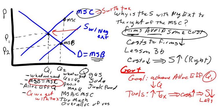
Price Ceiling (causes a
shortage)
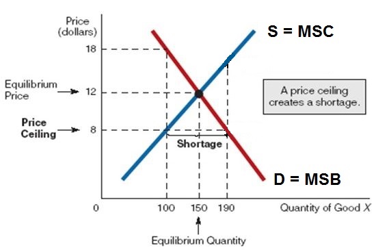
Price Floor (causes a
surplus)

Negative Externality
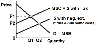
Negative Externality and
Taxes
- Price
Ceilings and Floors- Economics 2.6
[4:34 YouTube ACDC
Leadership]
- Pollution,
the Government, and MSB=MSC- Microeconomics
6.2
[3:25 YouTube ACDC Leadership]
- Micro
6.3 Negative Externalities: Econ Concepts in 60
Seconds-Externality
[2:31 YouTube ACDC Leadership]
NOTE: These are REVIEW videos only. In order to
learn the material you must read the assigned textbook readings,
watch the assigned lecture videos, and do problems. See the
MICWEBAPP
or the LESSONS
link for these assignments.
Unit 1: Markets are Efficient, Except
. . . Intro to Microeconomics
Lesson 5b: Market Failures Continued
(Positive Externalities and Public Goods)
We have learned in lessons 2a and 3c that
competitive markets are usually efficient. This is one of the
benefits of a market economy or capitalism. But sometimes markets
fail to be allocatively inefficient. In lesson 5a we learned that
when negative externalities exist, a market will produce too
much of a good or service (an overallocation of resources) and
therefore the government should tax the product (like gasoline taxes)
to get consumers to buy less, i.e. without the tax the price of
gasoline is too low.
In this lesson we will look at three other
market failures, positive externalities, public goods,
and the tragedy of the commons. With the first two the market
produces too little (an underallocation of resources) because the
demand curve for the product does not include all of the benefits.
The goal of government then is to increase production. With the
tragedy of the commons the market produces too much and the
goal of government is to reduce production.
Be careful. Remember, economists often change
the definitions of words. When we discuss "public goods" we do NOT
mean public schools, public parks, or public libraries. They are NOT
public goods according to our definition.
In later lessons (10 and 11) we will discuss
another market failure: the lack of competition. If a market
is not competitive, like when it is a monopoly or an oligopoly, then
profit maximizing businesses will produce less than the allocatively
efficient amount. The invisible hand of capitalism does not work well
if the market is not competitive.
When do product markets fail to be allocatively
efficient?
1. when there is not competition
(monopolies and oligopolies - lessons 10a, 10b, 11a, and 11b)
2. when the government sets the price (price ceilings and price
floors - lesson 5a)
3. when the supply curve does not include all
of the costs of producing or consuming the product (negative
externalities - lesson 5a)
4. when the demand curve does not include all of the benefits
of consumption (positive externalities - lesson 5b)
5. when the products are "public goods" (lesson 5b).
6. when there is a Tragedy of the Commons (lesson 5b)
5b Something Interesting - Why are we
studying this?
|
Why does the government do what it does?
Governments in the United States, build and run schools, libraries,
and parks, but not gas stations, clothing stores, or grocery stores?
Why some things and not other things? Does it make sense or is it
just random?
We have learned that competitve markets achieve
efficiency, both allocative and productive. And we learned that
competitive markets have a limited role for government. So why does
the government do schools, libraries, and parks, and we could add
roads, bridges, airports, football stadiums, and vaccinations. Why
these things and not other things? Why not let private businesses do
these things like they do gas stations, clothing stores, and grocery
stores?
If markets are efficient, then, if the
government is doing something rather than the market, WE SHOULD ASK,
WHY?
In this lesson you will learn two reasons that
explain much of why the government does what it does: POSITIVE
EXTERNALITIES and PUBLIC GOODS.
One other interesting question: public schools,
public libraries, and public parks ARE NOT PUBLIC GOODS. Why
not?
p. 84,
(19th, 93), "Market Failures in Competitive Markets"
pp.
90-100, (19th, 99-110), "Public Goods", "Externalities"
p. 400,
"Consider This: The Tragedy of the Commons"
Lecture
Outline
5b Assignments: Video
Lectures
|
MARKET FAILURE: POSITIVE
EXTERNALITIES
8.4.3 Explaining
How to Internalize External Benefits (Positive
Externalities (5:34)
[MyNotes]
Market
Failure - Positive Externalities of
Consumption (econclassroom.com
10:51)
MARKET FAILURE: PUBLIC GOODS
8.2.1 Defining
Public Goods 13:32
[MyNotes]
TRAGEDY OF THE COMMONS
The
Tragedy of the Commons as a Market Failure
(econclassroom.com 14:29) [MyNotes]
Tragedy
of the Commons (YouTube -
LearnLiberty - 3:19)
5b Outcomes - What you should
learn
|
TOPICS
- Positive Externalities (Spillover
Benefitrs, External Benefits)
- Public Goods
- Tragedy of the Commons
OUTCOMES
Market Failure: positive externalities (also
called external benefits or spillover benefits)
- define positive externalities (external
benefits or spillover benefits)
- give examples of positive
externalities
- use the MSB=MSC model to show the effects
on allocative efficiency of positive externalities
- what can the government do to correct the
market failure caused by positive externalities and show the
effects of these policies on the MSB=MSC model
- Demand is usually equal to MSB, but when
there are positive externalities the demand curve is to the left
of the MSB curve. Why?
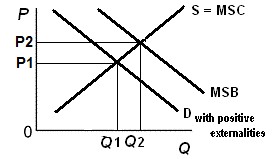
- Are positive externalities (spillover
benefits) good or bad for society? Why or why not?
- Comment on: EconMovies
7: Anchorman (Efficiency and Market Failures)
http://www.youtube.com/watch?v=FBjFDtH-iZM
Market Failure: Public Goods
- define "public goods (public goods are
non-exclusive and non-rival)"
- give examples of public goods and explain
why they are public goods
- define private (exclusive) goods" and give
examples
- define "rival goods" and give
examples
- what is the "free rider
problem"?
- explain how to derive the demand curve for
public goods
- what effect do public goods have on
allocative efficiency?
- what can the government do to correct for
the market failure of public goods?
- Why are public schools, public parks, and
public libraries NOT "public goods"? If they are not public goods
then why does the government produce them?
Market Failure: Tragedy of the
Commons
- what is the Tragedy of the Commons (common
access resources are non-exclusive but rival)
- how does the tragedy of the commons affect
allocative efficiency?
- what can be done to better achieve
allocative efficiency when there is a tragedy of the
commons?
Key Terms
Flash Cards - Click Here
Key Terms:
positive externalities (external
benefits or spillover benefits), private goods, public goods,
rivalry (rival goods), nonrival goods, excludability (exclusion
principle, exclusive goods), nonexcludability, (nonexclusive
goods), free-rider problem, benefit-cost analysis
(marginal-cost-marginal-benefit rule), tragedy of the commons,
common access resources
The
Economic Effects of Positive Externalities - Click
Here
Click on the link above to learn how to do this
problem.
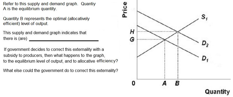
Positive Externalities (underallocationn
of resources)
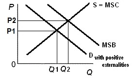
Positive Externalities and the Role of
Government: Increase Demand
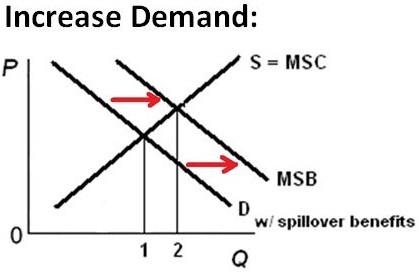
Positive Externalities and the Role of
Government: Increase Supply
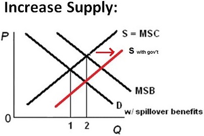
- Micro
6.4 Positive Externalities- ACDC Econ
[2:42 YouTube ACDC Leadership]
NOTE: These are REVIEW videos only. In order to
learn the material you must read the assigned textbook readings,
watch the assigned lecture videos, and do problems. See the
MICWEBAPP
or the LESSONS
link for these assignments.
Unit 2: Elasticity, Consumer Choice,
Costs
Lesson 4a: Price Elasticity of Demand
and Tax Incidence
We learned in lesson 3a that when the price of
pizza goes up the quantity demanded goes down. (What happens to
demand when price goes up? . . . . NOTHING.) So we know when the
price of a product goes up then the quantity demanded goes down, and
when the price goes down the quantity demanded goes up. We called
this the "law of demand" in lesson 3a. What we are going to learn in
lesson 4a is HOW MUCH?
If the price of pizza goes up, HOW MUCH
less will we buy? A LITTLE less or A LOT less? The price
elasticity of demand will answer this question and it will also
explain why farm incomes were high during a year of a record drought
and were low during a year of a record harvest.
You already understand elasticity. Think about
this:
If the price of gasoline goes up HOW
MUCH less will consumers buy? A little less or a lot less?
I believe most students will say A LITTLE less.
If the price of a Big Mac goes up, HOW MUCH
less will consumers buy? A little less or a lot less?
I bet most of you answered A LOT less.
If the price of salt goes up, how much less
will consumers buy? A little less or a lot less?
Correct. Only A LITTLE less.
If the price of a new car goes up, how much
less will consumers buy? A little less or a lot less?
A LOT less.
The price elasticity of demand measures
how responsive consumers are to changes in prices. Don't confuse
elasticity with the law of demand. The law of demand tells us that
when prices go up, the quantity demanded will go
down. Elasticity tells us HOW MUCH it will go down.
Lesson 3a - law of demand:
if the P
Qd
Lesson 4a - price elasticity of
demand:
if the P
does Qd or Qd
or Qd  ?
?
if price changes, HOW MUCH will the Qd change? A little or a
lot?
In lesson 3a we learned the direction of the
arrows (up or down). In lesson 4a we learn the size of the arrows
(big or small).
4a Something Interesting - Why are we
studying this?
|
In 2012 there was a severe drought in the US corn
growing region. In 2014 the weather was great and the corn crop was
at a record high. In which year did farmers make the most
money?
They made more in 2012 when the weather was bad
!!!
After studying this lesson you should
understand why good farming weather results in low farm incomes and
bad farming weather results in high farm incomes. Really!
See:
Sept. 2012: Despite
Record Drought, Farmers Expect Banner Year
Sept. 2014: Corn,
soybean crop expected to hit record high -- Great season could
mean bad prices for farmers ("This
year, farming income is expected to drop by 14
percent.")
ANSWER: The answer to this paradox is that the
demand for corn and soybeans is price INELASTIC. You will learn that
bad weather causes the price of crops to increase whch causes farm
incomes to increase and good weather causes the price of farm corps
to decrease causing incomes to decrease BECAUSE THE DEMAND FOR CORN
AND SOYBEANS IS PRICE INELASTIC.
pp. 134-143, (19th, 75-84), "Price Elasticity
of Demand'
pp. 146-147, (19th, 86-87), "Last Word -
Elasticity and Pricing Power: Why Different Customers Pay Different
Prices"
pp. 416-419, (19th, 347-354), "Tax Incidence
and Efficiency Loss"
Lecture
Outline
4a Assignments: Video
Lectures
|
2.4.1 Defining
Elasticity 4:47 [MyNotes]
2.4.2
Calculating
Elasticity 11:43 [MyNotes]
2.4.3
Applying
the Concept of Elasticity 8:42
[MyNotes]
2.4.4
Identifying
the Determinants of Elasticity 6:50
[MyNotes]
2.4.5
Understanding
the Relationship between Total Revenue and
Elasticity 8:09 [MyNotes]
Examining
the Effect of an Excise Tax on an Inelastic Good --
Cigarettes (econclassroom.com)
12:41
Examining
the Effect of an Excise Tax on an Elastic Good -- Candy
Bars (econclassroom.com)
8:08
OPTIONAL:
Calculating
and Interpreting Price Elasticity of Demand
(econclassroom.com ) 11:46
OPTIONAL: Price
Elasticity of Demand and the Total Revenue
Test (econclassroom.com)
13:24
4a Outcomes - What you should
learn
|
TOPICS
- price elasticity of demand
- tax incidence and efficiency
loss
OUTCOMES
- define price elasticity of
demand
- What is the difference between the "Law of
Demand" and the "Price Elasticity of Demand"?
- calculate the coefficient of price
elasticity of demand using the midpoint formula
- explain why the midpoint formula is
used
- know how to interpret the coefficient (what
does the number mean?)
- price elastic demand
- price inelastic demand
- unit elastic demand
- how does the price elasticity of demand
change along a single demand curve?
- perfectly price elastic demand
(graph)
- perfectly price inelastic demand
(graph)
- total revenue test (how do price changes
affect total revenue with different elasticities (show
graphically)
- P x Q = TR
- explain how the shape of the total revenue
graph is explained by the price elasticity of demand
- know the determinants of price elasticity
of demand and be able to use them to make an educated guess as to
whether a product has an elastic or inelastic demand
- Why might farm incomes fall if crops are
good (bumper crops)?
- how does the price elasticity of demand
explain the rise in street crime after a major drug
bust?
- how does price elasticity of demand help
explain how the minimum wage affects unemployment?
- define price discrimination and explain the
role of the price elasticity of demand
- define "excise tax" and give
examples
- understand the connection between price
elasticity of demand and the effect of excise taxes on (1) tax
incidence (burden), (2) tax revenue, and (3) allocative efficiency
(social welfare)
- explain the efficiency loss of excise taxes
using the (1) MSB = MSC model and (2) the consumer and producer
surplus model (dead weight loss)
- the role of excise taxes in income
redistribution and reducing negative externalities
- Use the concept of the price elasticity of
demand to answer these questions:
4a Determinants of Price Elasticity
of Demand and Supply
|
DETERMINANTS OF PRICE ELASTICITY OF
DEMAND
Number of Substitutes
Many
more price elastic
Few
less price elastic
Luxury or Necessity
Luxary
more price elastic
Necessity
less price elastic
Price of the product as a percent of sonsumer
income
Price is a large percent of consumer
income
more price elastic
price is a small percent of consumer income
less price elastic
Time
Long time between  price and when we measure quantity
more price elastic
price and when we measure quantity
more price elastic
Short time between
price and when we measure quantity
less price elastic
DETERMINANTS OF PRICE ELASTICITY OF
SUPPLY
Time
More time for producers to respond to
the
price
more price elastic
Less time for producers to respond to the
price
less price elastic
Ease of Storage
Easy and cheap to store the product
more price elastic
Difficult and expensive to store the product
less price elastic
Available Excess Capacity
A lot of extra room in the factory
more price elastic
Little extra room in the factory
less price elastic
Characteristics of the Production
Process
Easy to expand capacity
more price elastic
Difficult to expand capacity
less price elastic
Key
Terms Flash Cards - Click Here
Key Terms:
elasticity, price elasticity of
demand, midpoint formula, coefficient of price elasticity of
demand, price elastic demand, price inelastic demand, unit elastic
demand, perfectly elastic demand, perfectly inelastic demand,
total revenue, price discrimination, excise tax, tax incidence
(tax burden), efficiency loss of a tax, payroll tax
Calculate
Ed using the Midpoints Formula and Interpret the Results - Click
Here
Elasticity
and Total Revenue (TR) - Click Here
Elasticity
and the Incidence of Excise Taxes - Click Here
Click on the links above to learn how to do
these problems:
CALCULATE Ed USING MIDPOINTS
FORMULA
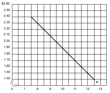
Calculate the price elasticity of demand
between a price of $2.40 and a price of $2.30 using the midpoints
formula and interpret the coeficient.
PRICE ELASTICITY OF DEMAND AND TOTAL
REVENUE
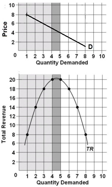
MULTIPLE CHOICE: Suppose that this total
revenue curve (see graph above) is derived from a particular linear
demand curve (see graph above). This demand curve must be:
A. inelastic for price declines that
increase quantity demanded from 6 units to 7 units.
B. elastic for price declines that increase quantity demanded from
6 units to 7 units.
C. inelastic for price declines that increase quantity demanded
from 4 units to 3 units.
D. elastic for price increases that reduce quantity demanded from
8 units to 7 units.
ELASTICITY AND INCIDENCE OF EXCISE
TAXES
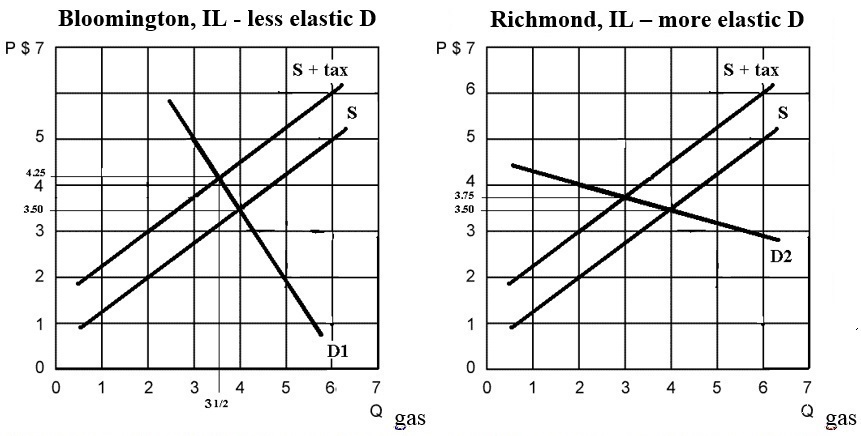
See the graphs above. Compare the following
when demand is more elastic (like in Richmond, IL on the
Wisconsin border), and less elastic (like in Bloomington IL in
the center of the state):
(1) incidence of the excise tax
(2) effect on allocative efficiency
(3) effect on government revenue
coefficient of price elasticity of demand
(midpoints formula)
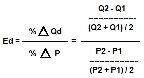
total revenue
TR = P x Q
Price Elasticity of
Demand
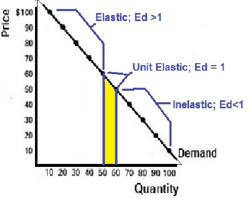
Total Revenue and Price Elasticity of
Demand
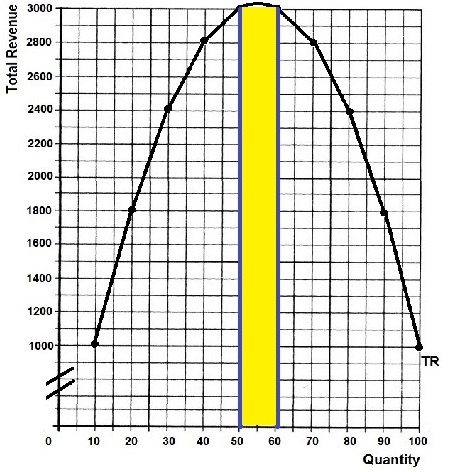
If the price decreases from $80 to $70
and
Total Revenue increases from $2400 to $2800,
then demand is price elastic.
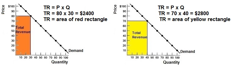
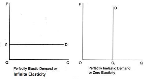
- Elasticity
and the Total Revenue Test- Micro 2.9
[6:13 YouTube ACDC Leadership]
NOTE: These are REVIEW videos only. In order to
learn the material you must read the assigned textbook readings,
watch the assigned lecture videos, and do problems. See the
MICWEBAPP
or the LESSONS
link for these assignments.
Unit 2: Elasticity, Consumer Choice,
Costs
Lesson 4b: Other Types of
Elasticity
Elasticity tells us HOW MUCH one variable changes
in response to a change in another variable. It is different than
demand and supply.
Demand - Lesson 3a:
If price increases what happens to the quantity demanded?
Supply - Lesson 3b:
If price increases what happens to the quantity
supplied?
Price elasticity of demand - Lesson 4a
If price increases HOW MUCH does the quantity demanded
decrease?
Price elasticity of supply - Lesson 4b:
If price increases HOW MUCH does the quantity supplied
increase?
We will study four different types of
elasticity:
1. price elasticity of demand (lesson
4a)
(If price changes, HOW MUCH does quantity demanded change?)
2. price elasticity of supply (lesson
4b)
(If price changes, how HOW MUCH does quantity supplied
change?)
3. cross elasticity of demand (lesson
4b)
(If the price of one product changes, HOW MUCH does the quantity
of another product change?)
4. income elasticity of demand (lesson
4b)
(If income changes, HOW MUCH does the quantity of a product
purchased change?)
4b Something Interesting - Why are we
studying this?
|
Ever wonder why the price of a computer printer
is so cheap and the price of ink cartridges for that printer are so
expensive? Stores sell printers at low prices because there is a
high and negative CROSS ELASTICITY OF DEMAND between printers
and ink. A company may offer a printer at a low price, because it
knows this will lead to increased sales for the highly profitable ink
cartridges. Printers and ink are complementary products.
The business term for this is "loss leader". A
business will sell one item at a loss to "lead" people into their
store who will buy lots of other related (complementary) items.
Before Thanksgiving in November the demand for
turkeys goes up so we would expect the price of turkeys to go up, but
if you have ever shopped for your Thanksgiving turkey you found that
they are usually on sale at low prices! Why?
The turkey is a loss leader. Selling turkeys at
a low price will bring more customers into the store who will buy
lots of other complementary items. This is because there is a high
and negative CROSS ELASTICITY OF DEMAND between turkeys and all
the other food we put on the Thanksgiving table.
pp. 143- 149, (19th, 84-89), "Price Elasticity
of Supply", "Cross and Income Elasticity of Demand"
Lecture
Outline
4b Assignments: Video
Lectures
|
PRICE ELASTICITY OF SUPPLY
Elasticity
of Supply (Khan Academy 9:33)
OPTIONAL
http://www.youtube.com/watch?v=nyKmrDYrkQ4
(YouTube TheWyvern66 9:48)
CROSS
ELASTICITY OF DEMAND
Cross
Elasticity of Demand (Khan Academy
11:20)
INCOME
ELASTICITY OF DEMAND
Income
Elasticity of Demand (YouTube Gale
Pooley 3:14)
4b Outcomes - What you should
learn
|
Price Elasticity of Supply
- define price elasticity of
supply
- calculate and interpret the coefficient of
price elasticity of supply using the midpoint formula
- determinants of price elasticity of
supply
- price elasticity of supply and the market
period, the short run, and the long run
- What is the difference between the "Law of
Supply" and the "Price Elasticity of Supply"?
Cross Elasticity of Demand
- define cross elasticity of
demand
- interpret the coefficient of cross
elasticity of demand including both its value and the sign
(substitutes, complements, and unrelated goods)
- Interpret this coefficient of cross
elasticity of demand: Eab = -2
Income Elasticity of Demand
- define income elasticity of
demand
- interpret the coefficient of income
elasticity of demand including both its value and the sign
(inferior goods, normal goods, luxury goods)
- Interpret this coefficient of income
elasticity of demand: Edy = + 0.5
4b Determinants of Price Elasticity
of Demand and Supply
|
DETERMINANTS OF PRICE ELASTICITY OF
DEMAND
Number of Substitutes
Many
more price elastic
Few
less price elastic
Luxury or Necessity
Luxary
more price elastic
Necessity
less price elastic
Price of the product as a percent of sonsumer
income
Price is a large percent of consumer
income
more price elastic
price is a small percent of consumer income
less price elastic
Time
Long time between
price and when we measure quantity
more price elastic
Short time between
price and when we measure quantity
less price elastic
DETERMINANTS OF PRICE ELASTICITY OF
SUPPLY
Time
More time for producers to respond to
the
price
more price elastic
Less time for producers to respond to the
price
less price elastic
Ease of Storage
Easy and cheap to store the product
more price elastic
Difficult and expensive to store the product
less price elastic
Available Excess Capacity
A lot of extra room in the factory
more price elastic
Little extra room in the factory
less price elastic
Characteristics of the Production
Process
Easy to expand capacity
more price elastic
Difficult to expand capacity
less price elastic
Key Terms
Flash Cards - Click Here
Key Terms:
price elasticity of supply,
coefficient of price elasticity of supply, midpoints formula,
market period, short run, long run, cross elasticity of demand,
substitute good, complement good, income elasticity of demand,
normal good, inferior good
Income
Elasticity of Demand
Cross
Elasticity of Demand
Click on the links above to watch these Key
Problems:
INCOME ELASTICITY OF DEMAND - MULTIPLE
CHOICE
1. Income elasticity of demand measures how
sensitive purchases of a specific product are to changes in:
A. the price of some other
product.
B. the price of that same product.
C. income.
D. the general price level.
2. The formula for income elasticity of demand
is percentage change in:
A. quantity demanded of X / percentage
change in price of X.
B. quantity demanded of X / percentage change in income.
C. quantity demanded of X / percentage change in price of Y.
D. price of X / percentage change in quantity demanded of
Y.
3. Which type of goods are most affected by
recessions (by a decrease in income)?
A. Goods for which the income
elasticity coefficient is relatively low.
B. Goods for which the income elasticity coefficient is relatively
high.
C. Goods for which the cross elasticity coefficient is
positive.
D. Goods for which the cross elasticity coefficient is
negative.
4. Suppose the income elasticity of demand for
boats is +2.0. This means that:
A. a 10 percent increase in income
will increase the purchase of boats by 20 percent.
B. a 10 percent increase in income will decrease the purchase of
boats by 20 percent.
C. a 10 percent increase in income will increase the purchase of
boats by 2 percent.
D. a 10 percent increase in income will increase the purchase of
boats by 2 percent.
5. Suppose the income elasticity of demand for
ramen noodles is -2.0. This means that:
A. a 10 percent increase in income
will increase the purchase of ramen noodles by 20 percent.
B. a 10 percent increase in income will decrease the purchase of
ramen noodles by 20 percent.
C. a 10 percent increase in income will increase the purchase of
ramen noodles by 2 percent.
D. a 10 percent increase in income will increase the purchase of
ramen noodles by 2 percent.
6. Suppose the income elasticity of demand for
electricity is +0.5. This means that:
A. a 10 percent increase in income
will increase the purchase of electricity by 50 percent.
B. a 10 percent increase in income will decrease the purchase of
electricity by 50 percent.
C. a 10 percent increase in income will increase the purchase of
electricity by 5 percent.
D. a 10 percent increase in income will increase the purchase of
electricity by 5 percent.
7. income elasticity can be used to tell if a
product is a normal good or inferior good. Which income elasticity
coefficient below indicates that the product is an inferior good?
A. Edy = +2.0
B. Edy = -2.0
C. Edy = +0.5.
D. Edy = 1.
8. income elasticity can be used to tell if a
product is a luxury or a necessity. Which income elasticity
coefficient below indicates that the product is a necessity?
A. Edy = +2.0
B. Edy = -2.0
C. Edy = +0.5.
D. Edy = -0.5.
CROSS ELASTICITY OF DEMAND - MULTIPLE
CHOICE
1. Cross elasticity of demand measures how
sensitive purchases of a specific product are to changes in:
A. the price of some other
product.
B. the price of that same product.
C. income.
D. the general price level.
2. The formula for cross elasticity of demand
is percentage change in:
A. quantity of X / percentage change
in price of X.
B. quantity of X / percentage change in income.
C. quantity of X / percentage change in price of Y.
D. price of X / percentage change in quantity demanded of
Y.
3. We would expect the cross elasticity of
demand between Pepsi and Coke to be:
A. negative and therefore these goods
are substitutes.
B. negative and therefore these goods are complements.
C. positive and therefore these goods are substitutes.
D. positive and therefore these goods are complements.
4. Suppose that a 20 percent increase in the
price of good Y causes a 10 percent decline in the quantity demanded
of good X. The coefficient of cross elasticity of demand is:
A. Negative (complements) and cross
elastic.
B. Negative (complements) and cross inelastic.
C. positive (substitutes) and cross elastic.
D. positive (substitutes) and cross inelastic.
5. Suppose the cross elasticity of demand for
Mobil gasoline and BP gasoline is +2.0. This means that:
A. a 10 percent increase in price of
Mobil gasoline will increase the purchase of BP gasoline by 20
percent.
B a 10 percent increase in price of Mobil gasoline will decrease
the purchase of BP gasoline by 20 percent.
C. a 10 percent increase in price of Mobil gasoline will increase
the purchase of BP gasoline by 2 percent.
D. a 10 percent increase in price of Mobil gasoline will decrease
the purchase of BP gasoline by 2 percent.
6. Suppose the cross elasticity of demand for
movie tickets and movie popcorn is -2.0. This means that:
A. a 10 percent increase in price of
movie tickets will increase the purchase of movie popcorn by 20
percent.
B. a 10 percent increase in price of movie tickets will decrease
the purchase of movie popcorn by 20 percent.
C. a 10 percent increase in price of movie tickets will increase
the purchase of movie popcorn by 2 percent.
D. a 10 percent increase in price of movie tickets will decrease
the purchase of movie popcorn by 2 percent.
7. Suppose the cross elasticity of demand for
butter and margarine is +0.5. This means that:
A. a 10 percent increase in the price
of butter will increase the quantity of margarine by 50
percent.
B. a 10 percent increase in the price of butter will decrease the
quantity of margarine by 50 percent.
C. a 10 percent increase in the price of butter will increase the
quantity of margarine by 5 percent.
D. a 10 percent increase in the price of butter will decrease the
quantity of margarine by 5 percent.
8. Cross elasticity can be used to tell if two
products are substitutes or complements. Which cross elasticity
coefficient below indicates that the products are complements?
A. Eab = +2.0
B. Eab = -2.0
C. Eab = +0.5.
D. Eab = 1.
coefficient of price elasticity of supply
(midpoints formula)
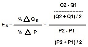
cross elasticity of demand
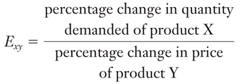
income elasticity of demand
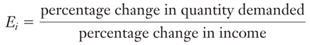
Perfectly Elastic and Inelastic
Supply
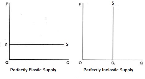
- Elasticity
of Demand Coefficients- Micro 2.10 (Cross-Price and Income
Elasticity)- AP Microeconomics
[7:02 YouTube ACDC Leadership]
NOTE: These are REVIEW videos only. In order to
learn the material you must read the assigned textbook readings,
watch the assigned lecture videos, and do problems. See the
MICWEBAPP
or the LESSONS
link for these assignments.
Unit 2: Elasticity, Consumer Choice,
Costs
Lesson 6a: Consumer Decisions: Utility
Maximization
When I go into the grocery store why do I buy 12
cans of pop, 3 frozen pizzas, and 1 pound of hamburger? Why don't I
buy 12 pounds of hamburger and 1 can of pop? In this lesson we will
use benefit-cost analysis to understand why we buy what we do. We
will calculate the marginal benefits (MB) of consuming something and
the marginal costs (MC) of consuming something. (Remember: all costs
in economics are opportunity costs.)
If our goal is to maximize our satisfaction we
will consume the quantity of goods and services where MB =
MC.
First, we will examine the benefits we get from
consumption. Economists call these benefits "utility". We will
calculate and graph total utility (TU) and marginal utility (MU). As
always, be sure you understand the SHAPES of these graphs. Remember:
Define, Draw, Describe.
Then, we will use the utility maximizing rule,
MUx/Px = MUy/Py = MUz/Pz = . . . ,
to calculate how much we should buy in order to
maximize our satisfaction (utility).
Be sure that you can see that the utility
maximizing rule is really just a version of benefit cost analysis,
MB=MC. If I am thinking about going skiing today, the MB would be the
extra utility that I get from a day of skiing: MBskiing = MUskiing.
Since all costs are opportunity costs, the marginal cost of skiing
would be the utility that I would lose because I am not doing
something else like going to a movie with my wife: MCskiing =
MUmovie.
Finally, why do we divide the MU by the price?
It doesn't make sense to compare a $45 ski ticket with a $12 movie
ticket. By dividing by price we end up comparing $1 worth of skiing
with $1 worth of a movie.
So, to maximize my utility I should go skiing
and go to movies with my wife so that the:
MUskiing/Pskiing=
MUmovie/Pmovie.
Even though MUx/Px = MUy/Py looks
different than MBx=MCx, it is really the same thing. Be sure
you do the exercises in the yellow pages.
6a Something Interesting - Why are we
studying this?
|
In October and November ski resorts in the west
begin to open with just a few runs open and large crowds of skiers
and snowboarders. In late April most western ski areas have a lot of
snow and are mostly 100% open but few skiers and snowboarders come.
Why? Why are there so many customers when the snow is bad in the fall
and so few when the snow is good in the spring?
Read the following from an online skiing
discussion forum: http://www.epicski.com/t/39322/skiing-in-past-march-why-not-popular
Note: "PNW" means the "Pacific northwest" (i.e. the states of Oregon
and Washington).
The skier asks, "But, for some reason, people
just stop skiing (in April). WHY? I just don't understand." After
studying this lesson you should be able to explain WHY to the skier
who posted on the forum.
Here is another interesting question: Why do
pop vending machines allow you to only get one can at a time while
newspaper vending machines allow you to take as many as you want when
you only pay for one?
ANSWER: The answer to both questions has to do
with the "law of diminishing marginal utility".
pp. 152-162, (19th, 116-125), " Law of
Diminishing Marginal Utility", "Theory of Consumer Behavior",
"Utility Maximization and the Demand Curve", "Income and Substitution
Effects", "Applications and Extensions"
Lecture
Outline
6a Assignments: Video
Lectures
|
3.1.1 Understanding
Utility Theory 4:31
[MyNotes]
Plotting
MU at the Midpoint (4:50)
3.1.2
Finding
Consumer Equilibrium - The Utility Maximizing Quantities to
Buy 4:47 [MyNotes]
Professor
Harmon Calculates the Utility Maximizing Bundle in 5
mins (YouTube - 02001orh)
4:58
6a Outcomes - What you should
learn
|
TOPICS
- diminishing marginal utility
- utility maximization
OUTCOMES
- Define, Draw, and Describe the total
utility and marginal utility graphs
- Understand the relationship between the
total utility and marginal utility graphs
- Understand the law of diminishing marginal
utility.
- Describe how rational consumers maximize
utility by using benefit-cost-analysis. (Utility maximizing rule;
MUx/Px = MUy/Py = MUz/Pz )
- Explain how a demand curve can be derived
by observing the outcomes of price changes in the
utility-maximization model
- If lobster was free and if lobster was your
favorite food, would you eat lobster for every meal everyday? Why
or why not?
- Why do pop vending machines allow you to
only get one can at a time while newspaper vending machines allow
you to take as many as you want when you only pay for
one?
- Why do we have to divide by price in the
utility maximizing rule?
- Benefit Cost Analysis: MB =
MC
- Utility Maximizing Rule: MUa/Pa =
MUb/Pb
Key Terms
Flash Cards - Click Here
Key Terms:
utility, total utility (TU), marginal
utility (MU), law of diminishing marginal utility, rational
behavior, benefit-cost analysis, budget constraint,
utility-maximizing rule, marginal utility per dollar (MU/P),
"util", income effect, substitution effect, diamond-water
paradox
How
to plot MU at the midpoint - Click Here
How
to find the Utility Maximizing Quantities to Buy - Click
Here
Click on the links above to learn how to do
these problems:
HOW TO PLOT MARGINAL UTILITY (MU) AT THE
MIDPOINT
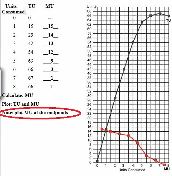
HOW TO FIND THE UTILITY MAXIMIZING
QUANTITIES TO BUY
Use the data below to calculate the utility
maximizing quantities to buy (What quantities would a rational
consumer buy?) AND what is the maximum total utility (TU)
possible?
Assume the price of X is $2 and the price of Y
is $4. The consumer has $20 of income to spend.
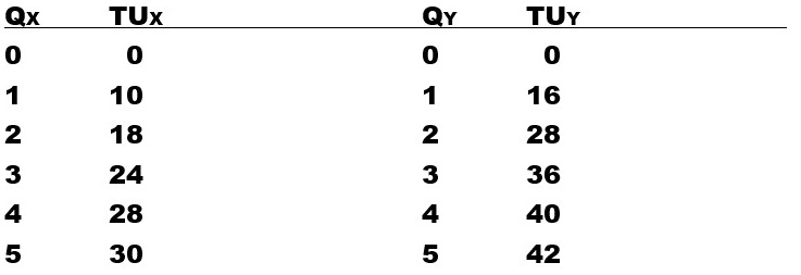
marginal utility
MU =  TU /
Qconsumed
TU /
Qconsumed
benefit-cost analysis
MB = MC
utility-maximizing rule
MUa/Pa = MUb/Pb = MUc/Pc = . . .
Total Utility (TU) and Marginal Utility
(MU).
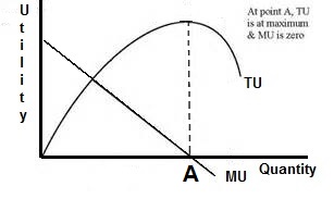
Remember: the marginal is the slope of the
total. The slope of the TU curve is getting smaller and smaller
(less steep) as the quantity consumed increases. At the same time
MU is less and less. At its peak the slope of the TU curve is zero
and at this quantity MU is zero (it crosses the X
axis).
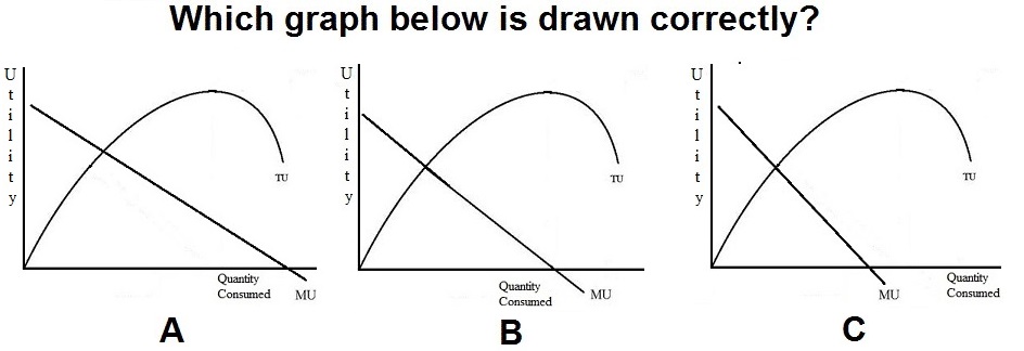
- Micro
2.12 Utility Maximization: Econ Concepts in 60 Seconds - Diminishing
Marginal Utility
[2:10 YouTube ACDC Leadership]
NOTE: These are REVIEW videos only. In order to
learn the material you must read the assigned textbook readings,
watch the assigned lecture videos, and do problems. See the
MICWEBAPP
or the LESSONS
link for these assignments.
Unit 2: Elasticity, Consumer Choice,
Costs
Lesson 7a: Economic Profit and the
Production Function
In lessons 7, 8/9, 10, and 11 we will be looking
at the producer decision of HOW MUCH TO PRODUCE. We will use benefit
cost analysis (MB=MC) to find the profit maximizing quantity or WHAT
WE GET. Once we know how much businesses will produce, we will ask:
Is this quantity WHAT WE WANT? (Is this quantity efficient - both
allocatively and productively)?
To find the profit maximizing quantity we will
use benefit-cost analysis: MB=MC. So, what are the extra benefits of
producing one more unit of output? How do businesses benefit when
they produce one more? Well, they get more money, called revenue.
Even if they are earning losses, they receive more revenue when they
sell more. The extra revenue that businesses get when they produce
and sell one more unit is their marginal revenue (MR). This is the MB
of producing one more.
But there are also extra costs of producing one
more unit of output. We call these the marginal costs (MC). When
MR=MC (MB=MC) their profits will be maximized. NOTE: when MR=MC
profits are not necessarily zero, but they are as large as possible.
We will calculate these profits in lessons 8/9, 10, and
11.
In lessons 7a, 7b, and 7c we begin by looking
at the MC. Then in lessons 8/9, 10, and 11 we add the MR.
In lessons 7a, 7b, and 7c we will introduce
three new sets of graphs. First (lesson 7a) we will look at the
production function thast shows how output changes when we add more
resources. We will then (lesson 7b) use the production function graph
to understand the SHAPES of the other two sets of graphs. The two
sets of cost graphs show us what happens to costs when we produce
more. These two sets of cost graphs are the total cost graphs (TC,
TVC, and TFC) and the average cost graphs (ATC, AVC, AFC, and
MC).
Let's begin with the production function, or
HOW DOES OUTPUT CHANGE WHEN WE ADD MORE RESOURCES?
One more thing. If a firm is earning zero
economic profits, that is OK!!! But a zero economic profit is NOT the
same as a zero accounting profit. A zero economic profit could be an
accounting profit of $1 million dollars a year! Be sure you learn the
difference between an "economic profit" and an "accounting profit"
and understand WHY the difference exists. (Hint: It has to do with
the fact that economists always use "opportunity costs" and
accountants don't.)
7a Something Interesting - Why are we
studying this?
|
Assume your GPA is 3.0, a "B" average. Let's call
the GPA that you earn this semester your MARGINAL grade point
(MGP; Remember "marginal" means "extra".)
What happens to your 3.0 GPA if you get
straight C's this semester? (What happens to your grade point
AVERAGE, 3.0 if your MARGINAL grade point, 2.0, is lower?)
What happens to your 3.0 GPA if you get
straight A's (4.0) this semester? (What happens to your grade point
AVERAGE if your MARGINAL grade point is higher?)
What happens to the AVERAGE Product (AP) if the
MARGINAL Product (MP) is above it? ANSWER: if MP is greater than AP
then AP will rise.
What happens to the AVERAGE Product (AP) if the
Marginal Product (MP) is below it? ANSWER: if MP is less than AP then
AP will fall.
Marginal Product curve crosses the Average
Product curve where?
For all graphs: DEFINE, DRAW, DESCRIBE the
shape.
pp. 196-202, (19th, 140-147), "Economic Costs",
"Short-Run Production Relationships"
Lecture
Outline
7a Assignments: Video
Lectures
|
AN ECONOMIST'S VIEW OF COSTS AND
PROFIT
5.1.4 Finding
Economic and Accounting Profit 13:54
[MyNotes]
PRODUCTION
IN THE SHORT RUN
4.1.1 Understanding
Output, Inputs, and the Short Run
8:48 [MyNotes]
4.1.2 Explaining
the Total Product Curve 15:57
[MyNotes]
4.1.3
Drawing
Marginal Product Curves 7:22
[MyNotes]
How
to Plot MP at the Midpoint
6:54
4.1.4
Understanding
Average Product 10:32
[MyNotes]
7a Outcomes - What you should
learn
|
TOPICS
- accounting and economic profits
- production function: how output changes
with inputs
OUTCOMES
- Distinguish between explicit and implicit
costs, and between accounting and economic profits
- Explain why a normal profit is an economic
cost, but an economic profit is not
- Why is a zero economic profit OK for
businesses?
- What are sunk (fixed) costs and why are
they ignored?
- Explain the law of diminishing (marginal)
returns
- Differentiate between the short run and the
long run.
- Compute and graph marginal product and
average product when given total product data
- Explain the relationship between total
product, marginal product, and average product
- Explain the shape of the total product,
marginal product, and average product graphs (specialization and
teamwork, congestion, and overcrowded)
- Differentiate between production,
productivity, and productive efficiency
- Explain what is meant by: the MP curve is
the slope of the TP curve
(Note: All marginal curves are the slopes of their total
curves.)
- Assume your GPA is 3.0:
- What happens to your GPA if your you get
straight C's (2.0) this semester?
- What happens to your GPA if your you get
straight A's (4.0) this semester?
- What happens to the AP curve if the MP
is above it?
What happens to the AP curve if the MP is below it?
Key
Terms Flash Cards - Click Here
Key Terms:
economic cost, explict cost, implicit
cost, accounting profit, economic profit, normal profit,
production function, short run, long run, total product (TP),
marginal product (MP), average product (AP), law of diminishing
returns, increasing marginal returns, diminishing marginal
returns, negative marginal returns, specialization and teamwork,
congestion (getting crowded), overcrowded,
productivity vs. production vs. productive
efficiency
How
to plot MP at the midpoint - Click Here
Calculate,
Plot, and Describe TP, MP, AP
Click on the links above to learn how to do
this problem:
HOW TO PLOT MARGINAL VALUES AT THE
MIDPOINT
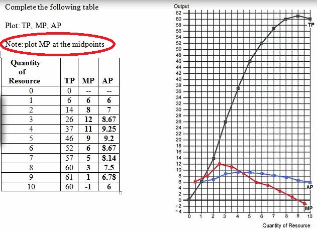
CALCULATE, PLOT, and DESCRIBE TP, MP,
AP
Use the data below to:
Graph the quantity produced (total product,
TP)
Calculate and graph marginal product (MP) at the midpoints.
Calculate and graph average product (AP).
Describe (explain) the shape of the TP and MP graphs.
Describe (explain) the shape of the AP and MP graphs.
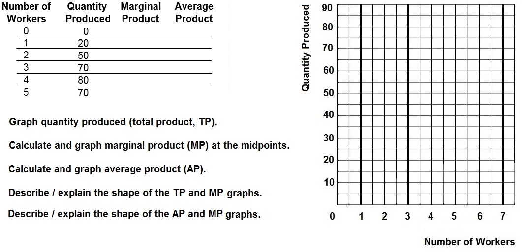
accounting profit
acct. profit = total revenues
- explicit costs
economic profit
econ. profit = total revenue -
(expicit costs + implicit costs)
marginal product (MP)
MP =
TP /
Qres
average product (AP)
AP = TP / Qres
The Production Function: Total Product
(TP), Average Product (AP), and Marginal Product
(MP)
NOTICE:
The marginal is the slope of the
total.
The slope of the TP curve gets bigger
(steeper) at first then it gets smaller and smaller (less
steep) as the quantity of the resources increases. At the same
time MU at first goes up then gets less and less. At its peak
the slope of the TP curve is zero and at this quantity MP is
zero (it crosses the X axis). MP is at its highest when TP is
at its steepest point.
MP crosses AP when AP is at its peak.
Another way of saying this is when MP is above AP, then AP is
increasing. When MP is below AP then AP is
decreasing.
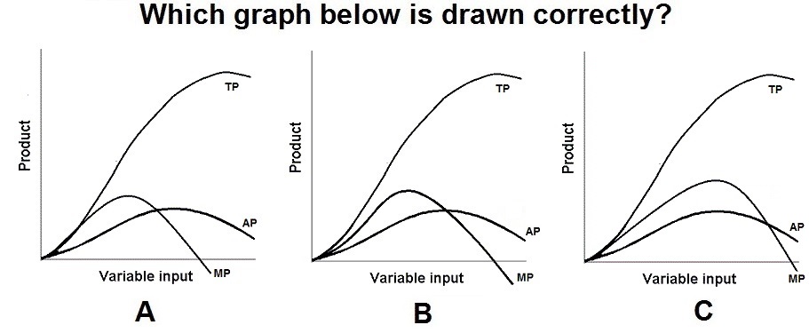
- Economic
Profit and Costs- ACDC Econ - Micro 3.6
[3:47 YouTube ACDC Leadership]
- Diminishing
Marginal Returns- Micro 3.1
[5:53 YouTube ACDC Leadership]
- Micro
3.1 The Law of Diminishing Marginal Returns - Econ Concepts in 60
Seconds (YouTube, ACDC Leadership
5:30)
NOTE: These are REVIEW videos only. In order to
learn the material you must read the assigned textbook readings,
watch the assigned lecture videos, and do problems. See the
MICWEBAPP
or the LESSONS
link for these assignments.
Unit 2: Elasticity, Consumer Choice,
Costs
Lesson 7b: Production Costs in the
Short Run
7b Introduction
|
|
OK. Now that we know about (1)
specialization and teamwork, (2) getting crowded, and (3)
overcrowded, from lesson 7a, that is, we know why the TP
curve has the shape that it does, we are ready to look at
the graphs that we will be using most in this class: the
cost curves (both total and average). Remember, we are
studying economic costs so that we can calculate the MC -
the extra costs of producing one more unit of output. In
lessons 8/9, 10, and 11 we will combine MC with MR (the
extra benefits of producing and selling one more unit of
output ) so that we can find the profit maximizing quantity
of output, or the quantity where MR=MC. This is WHAT WE
GET.
The costs curves show us how costs
change with output. The production function in lesson 7a
showed us how output changes when we add more resources.
They are related. We studied the production function so that
we could learn about (1) specialization and teamwork, (2)
getting crowded, and (3) overcrowded, because these concepts
will help us understand the shapes of the cost curves.
Remember: whenever we learn a new graph we must understand
it shape (For all graphs: DEFINE, DRAW, DESCRIBE its
shape).
In this lesson we will be looking at
the SHORT RUN COST CURVES. We studied the definition of
"short run" in lesson 4b. It doesn't really have much to do
with time. The short run in some industries is longer than
the long run in other industries. In the short run the
quantity of at least one resource is fixed, does not change.
We will usually assume that the number of factories or the
size of the factory does not change. So in the short run we
are adding more resources to an EXISTING factory . . . and
it may get crowded or overcrowded. We will look at the long
run costs (when we can change the number of factories or the
size of the factories) in the next lesson, 7c.
Finally, we will be looking at three
types of costs: fixed, variable, and total (total equals
fixed plus variable), and three "families" of costs: total,
average, and marginal. By the end of this lesson you should
be able to correctly Calculate, Define, Draw, and Describe
the shapes of: TFC, TVC, TC, AFC, AVC, ATC, and MC. (For all
graphs: DEFINE, DRAW, DESCRIBE its shape).
|
pp. 202-209, (19th, 147-152), "Short-Run
Production Costs"
Lecture
Outline
7b Assignments: Video
Lectures
|
4.1.5 Relating
Costs to Productivity 5:26
[MyNotes]
4.2.1
Defining
Variable Costs 4:23 [
[MyNotes]
4.2.2
Graphing
Variable Costs 4:57
[MyNotes]
4.2.3
OPTIONAL: Graphing
Variable Costs Using a Geometric Trick
5:04
4.3.1
Defining
Marginal Costs 6:41
[MyNotes]
4.3.2
Deriving
the Marginal Cost Curve 10:59
[MyNotes]
4.3.3
Understanding
the Mathematical Relationship between Marginal Cost and Marginal
Product 10:26 [MyNotes]
4.4.1
Defining
Average Variable Costs 5:39
[MyNotes]
4.4.2
OPTIONAL: Understanding
the Relationship between Average Variable Costs and Average
Product 6:06 [MyNotes]
4.4.3
Understanding
the Relationship between Marginal Cost and Average Variable
Cost 7:54 [MyNotes]
4.5.1
Defining
and Graphing Average Fixed Cost and Average Total
Cost 6:55 [MyNotes]
4.5.2
Calculating
Average Total Cost 4:50
[MyNotes]
4.5.3
Putting
the Cost Curves Together 10:09
[MyNotes]
4.6.4
Shifts
in the Cost Curves 4:49
[MyNotes]
7b Outcomes - What you should
learn
|
TOPICS:
- Short Run Costs: Define Draw,
Describe
OUTCOMES:
- Distinguish between fixed, variable and
total costs:
- Explain the difference between average and
marginal costs
- Compute and graph AFC, AVC, ATC, and MC
when given total cost data
- Know how and why we graph the MC "at the
midpoints".
- Explain how TC, TVC, and TFC relate to one
another: Do TC and TVC get closer
together?
- Explain how AVC, ATC, and MC relate to one
another
- do ATC and AVC get closer
together?
- why does MC cross ATC and AVC at their
lowest points?
- Explain the shapes of the total, average,
and marginal cost curves (TC, TVC, TFC, ATC, AVC, AFC, and
MC)
- Relate average product to average variable
cost, and marginal product to marginal cost
- Explain what happens to the cost curves if
there is a change in fixed costs and what happens if there is a
change in variable costs (what can cause cost curves to rise or
fall?)
Key Terms
Flash Cards - Click Here
Key Terms:
short run, fixed costs, variable
costs, total fixed cost (TFC), total variable cost (TVC), total
cost (TC), average fixed cost (AFC), average variable cost (AVC),
average total cost (ATC), marginal cost (MC)
Graph
TC, TVC, TFC and ATC, AVC, MC (YP
40)
On
a Graph with Numbers find TC, TVC, TFC, ATC, AVC, AFC,
MC (YP 38-39)
On
a Graph with Letters (geometry) find TC, TVC, TFC, ATC, AVC, AFC,
MC (YP 44)
How
to find TVC on a graph with letters given AVC - Click
Here
On a Graph with Numbers find TC, TVC, TFC,
ATC, AVC, AFC, MC
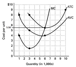
On a Graph with Letters (geometry) find TC,
TVC, TFC, ATC, AVC, AFC, MC
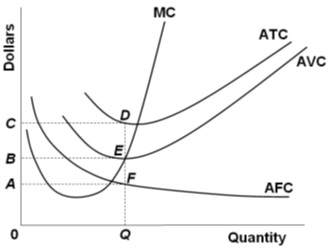
How to find TVC on a graph with letters
given AVC
Use the figure below. If output equals 0n, what
are the total variable costs (TVC)?
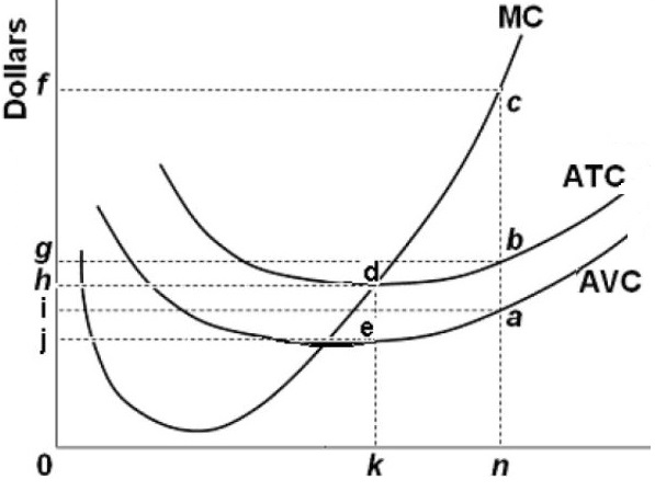
AFC = TFC / Q
AVC = TVC / Q
ATC = TC / Q
AFC + AVC = ATC
TFC + TVC = TC
MC = TC
/
Q
Total Cost Curves:
Total Cost TC, Total Variable Cost,
(TVC), Total Fixed Cost (TFC)
Average Cost Curves and Marginal Cost:
Average Total Cost (ATC) , Average
Variable Cost, (TVC), AverageFixed Cost AFC), and Marginal Cost
(MC)
NOTICE: MC crosses ATC and AVC at their
lowest points
Which graph
below is drawn correctly?
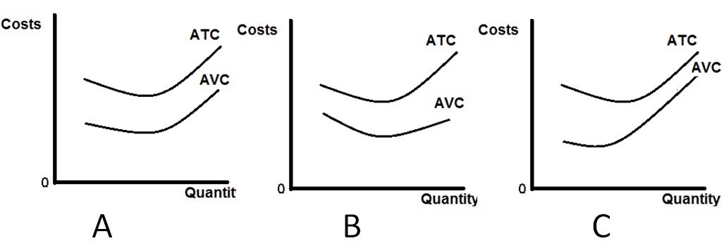
Which colored rectangle below is largest
(assume the ATC and AVC curves are identical)?
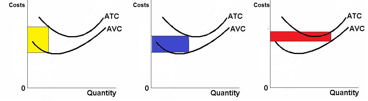
- Micro
3.2 AP Economics - Marginal Product and Marginal Cost: Econ concepts
in 60 Seconds Review [YouTube ACDC
Leadership, 4:54]
- Costs
of Production- Microeconomics 3.3 (Part 1)
[5:16 YouTube ACDC Leadership]
- Cost
Curves- Microeconomics 3.3 (Part 2)
[3:13 YouTube ACDC Leadership]
- Marginal
Cost and Average Total Cost- Micro 3.4
[3:16 YouTube ACDC Leadership]
- Micro
3.5 AP Economics Marginal Product and Marginal Cost: Econ Concepts in
60 Seconds Review [4:54 YouTube
ACDC Leadership]
- Marginal
Cost and ATC - Why do cost curves do that?
[YouTube, ACDC Leadership, 3:16]
- How
to find TVC on a graph with letters
[Screencast by your instructor]
NOTE: These are REVIEW videos only. In order to
learn the material you must read the assigned textbook readings,
watch the assigned lecture videos, and do problems. See the
MICWEBAPP
or the LESSONS
link for these assignments.
Unit 2: Elasticity, Consumer Choice,
Costs
Lesson 7c: Production Costs in the
Long Run
In lesson 7b we calculated and graphed SHORT RUN
costs when the size of the factory was fixed (did not change). Here
we will learn how costs change in the LONG RUN. In the long run we
can change the size of the factory. Only in the long run can new
firms enter an industry and only in the long run can firms leave the
industry (go out of business). Be sure that you can define "short
run" and "long run".
As always, be sure you know why the long run
ATC curve has the shape it does; For all graphs: DEFINE, DRAW,
DESCRIBE the shape.
Note that in the next unit (unit 3) we will use
long run graphs to find the allocatively efficient quantity and the
productively efficient quantity.
7c Something Interesting - Why are we
studying this?
|
Why are there many hardware stores in Illinois
but only two automobile production plants?
ANSWER: The answer has to do with the different
shapes of the long run ATC curve for retail stores and for automobile
production.
pp. 209-216, (19th, 152-162 ), "Long-Run
Production Costs", "Applications and Illustrations"
Lecture
Outline
7c Assignments: Video
Lectures
|
4.6.1 Defining
the Long Run 5:55 [MyNotes]
4.6.2
Determining
the Firm's Return to Scale 9:01
[MyNotes]
4.6.3 Understanding
the Short Run and Long Run Average Cost Curves
15:06 [MyNotes]
7c Outcomes - What you should
learn
|
TOPICS:
- The Long-Run ATC Curve
- Economies of Scale and Industry
Structure
OUTCOMES:
- Explain the difference between short run
and long run costs
- State why the long run average cost is
expected to be U shaped
- List and explain the causes of economies
and diseconomies of scale
- Indicate the relationship between economies
of scale and number of firms in an industry and their
sizes
- Why are there many hardware stores in
Illinois but only two automobile production plants?
Key
Terms Flash Cards - Click Here
Key Terms:
short run, long run, economies of
scale, diseconomies of scale, constant returns to scale, minimum
efficient scale, natural monopoly
- Economies
of Scale- Micro 3.2
[3:54 YouTube ACDC Leadership]
NOTE: These are REVIEW videos only. In order to
learn the material you must read the assigned textbook readings,
watch the assigned lecture videos, and do problems. See the
MICWEBAPP
or the LESSONS
link for these assignments.
Unit 3: Are Businesses Efficient?
Product Markets and Efficiency
Lesson 8/9a: Pure Competition:
Characteristics and Short Run Equilibrium
ARE BUSINESSES EFFICIENT?
In lessons 8/9, 10, and 11 we will be looking
at the producer decision of HOW MUCH TO PRODUCE. We will use benefit
cost analysis (MB=MC) to find the profit maximizing quantity which is
WHAT WE GET. Once we know how much businesses will produce, we will
ask: Is this quantity efficient (both allocatively and productively)
which is WHAT WE WANT.
We already know that businesses will maximize
profits when they produce the equilibrium quantity where Qs=Qd
(lesson 3c). We also know that for competitive markets this will be
the efficient quantity (except in a few situations where the market
fails - lessons 5a and 5b).
Keep in mind that there are thousands of
business firms. And when a business starts they do not look at an
economics textbook to see what model they want to be in. With only
four product market models many businesses will not fit exactly into
one of the four models. Think of the four product market models as a
continuum (see below) with pure competition on one end and pure
monopoly on the other end and all businesses will fall somewhere
in-between even though they my not fit neatly into any one single
model.
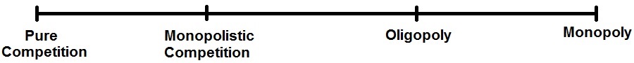
We will begin by looking at competitive markets
in lessons 8/9a and 8/9b. We should not be surprised that in
competitive markets when businesses produce the profit maximizing
quantity, they will also be producing the allocatively and
productively efficient quantities. Competitive markets are
efficient.
There are few real world examples of
competitive industries. Agriculture comes close. But, we do not study
pure competition just to understand agriculture. We study pure
competition because IF it did exist then it would be efficient (both
allocatively and productively). Pure competition then helps us to
better learn what efficiency means. Once we know this, we will study
the "real world" in lessons 10a, 10b, 11a, 11b and compare the real
world with a competitive world. We therefore use pure competition as
a standard against which we can compare the real world, a standard of
efficiency.
For each of the four product market models
(lessons 8-11) you should use the following general outline to guide
your studying:
General Outline for Each Product Market
Model:
1. Know the model's characteristics
and examples (See the "8/9a QUIZ - 4 PRODUCT MARKETS" quiz on our
Blackboard site.)
2. Be able to explain the shape of the demand curve
3. Draw the short run equilibrium graphs for (a) profit maximizing
firms, (b) loss minimizing firms, and (c) firms that will shut
down
4. Draw the long run equilibrium graph and find the profit
maximizing quantity (WHAT WE GET), allocatively efficient quantity
(WHAT WE WANT), and the productively efficient quantity. See the
last 13 pages of the Unit 3 Yellow Pages ("3 Rules and 4
Models").
5. Understand any other issues associated with the model
Never forget this: To maximize profits
business will produce the quantity where MR=MC.
8/9a Something Interesting - Why are
we studying this?
|
Click on the link below and read the answer
to these questions.
- Why must MC=MR to achieve the
maximum profit or to have the lowest loss?
- Why must Marginal Cost be equal to
Marginal Revenue? Won't that earn nothing?
 Yahoo!
Answers: Profit Maximizing Question - MC=MR?
Yahoo!
Answers: Profit Maximizing Question - MC=MR?
ANSWER: Whenever you are asked questions
like:
- "what quantity will be produced?",
- "what price will be charged?",
- "what is the profit maximizing quantity?",
- "what is the equilibrium quantity?", etc.,
the first thing you do is calculate MR and
MC.
Then, as long as the firm earns more (MR) than
it costs (MC) they will produce. They will produce ALL where
MR>MC, up to where MR=MC, but never where MR<MC.
8/9a Assignments:
Readings
|
pp. 220-238, ALL, (19th, Ch. 8, ALL),"Pure
Competition in the Short Run"
PRACTICE QUIZ - 8/9a - on Blackboard
Lecture
Outline
8/9a Assignments: Video
Lectures
|
MARKET STRUCTURE
5.1.3 Understanding
Market Structure 10:55
[MyNotes]
WHAT IS A
PERFECTLY COMPETITIVE MARKET? (PURE COMPETITION)
5.1.2 Understanding
the Role of Price 3:43
[MyNotes]
5.1.1
Calculating
Total Revenue 3:36 MyNotes]
PURE
COMPETITION - SHORT RUN PROFIT MAXIMIZATION
5.2.1 Finding
the Firm's Profit Maximizing Output Level
14:24 [MyNotes]
5.2.2
Proving
the Profit Maximizing Rule 4:20
[MyNotes]
5.2.3
Calculating
Profit 12:26 [MyNotes]
5.2.4
Calculating
Loss 9:13 [MyNotes]
5.2.5
Finding
the Firm's Shut-Down Point 8:35
[MyNotes]
PURE
COMPETITION - SHORT AND LONG RUN MARKET SUPPLY
5.3.1 Deriving
the Short-Run Market Supply 20:44
[MyNotes]
8/9a Outcomes - What you should
learn
|
TOPICS
- characteristics of the four product market
models
- pure competition - short run
equilibrium
OUTCOMES
- List the four basic market models and know
characteristics and examples of each.
- Describe characteristics and examples of a
purely competitive firms and industries.
- Explain how a purely competitive firm views
demand for its product and marginal revenue from each additional
unit sale. Why is the demand curve horizontal (perfectly price
elastic) for purely competitive firms?
- Compute and graph average revenue (also
called price), total revenue, and marginal revenue when given a
demand schedule for a purely competitive firm.
- Use both total revenue minus total cost
approach and the marginal revenue = marginal cost approach to
determine the short run price and output that maximizes profits
(or minimizes losses) for a competitive firm.
- with a table of data
- on a graph with numbers
- on a graph using geometry (graph with
letters)
- Draw the short run equilibrium graphs for a
purely competitive firm that (a) maximizes profit, (b) minimizes
loss, and (c) shuts down
- If MR = MC, what will a firm's profits
be?
Key Terms
Flash Cards - Click Here
Key Terms:
pure competition, pure monopoly,
monopolistic competition, oligopoly, imperfect competition,
standardized (homogenous) product, differentiated product,
nonprice competition, perfectly elastic demand, market power,
price taker, average revenue (usually price), marginal revenue,
total revenue, MR=MC rule (profit maximization rule), short-run
equilibrium, short-run supply curve
Finding
the profit maximizing quantity on a table - 1 - Click
Here
Finding
the profit maximizing quantity on a table - 2 - Click
Here
[works for me if I save the file to my computer first, then open
it[
Finding
the profit maximizing quantity on a graph with numbers - Click
Here
Finding the profit maximizing quantity on
a table - 1
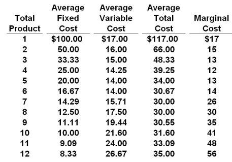
1. MULTIPLE CHOICE: Refer to the above data. If
the market price for the firm's product is $12, the competitive firm
will produce:
A. 4 units at a loss of $109
B. 4 units at an economic profit of $31.75
C. 8 units at a loss of $48.80
D. zero units at a loss of $100
Finding the profit maximizing quantity on
a table - 2
Answer this question on the basis of the
following cost data for a purely competitive seller.
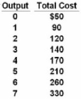
MULTIPLE CHOICE: Refer to the above data. If
the product price is $45, the firm will:
A. shut down
B. produce 4 units and realize and $120 economic profit
C. produce 5 units and realize and $15 economic profit
D. produce 6 units and realize and $100 economic profit
Finding the profit maximizing quantity on
a graph with numbers
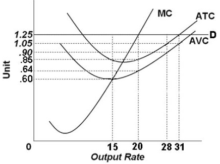
MULTIPLE CHOICE: What is the profit maximizing
level of output?
A. 15
B. 31
C. 28
D. 20
Profit = TR - TC
TR = P X Q = AR x Q
AR = TR / Q = P = Average Revenue
MR = TR
/ Q
Profit Maximization Rule: MR=MC
Pure Competition: The Demand
Curve
Pure Competition: Short Run Earning
Profits

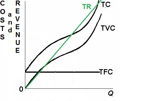
Pure Competition: Short Run Earning
Losses
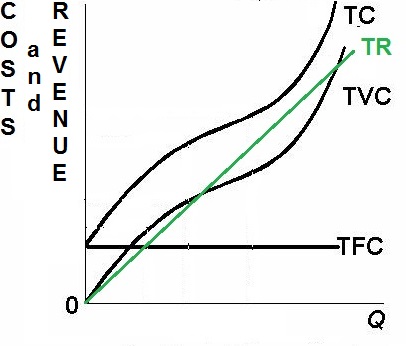
Pure Competition: Short Run Shut
Down
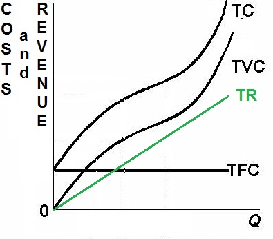
- Perfect
Competition in the Short Run- Microeconomics 3.8
[4:49 YouTube ACDC
Leadership]
- Micro
3.7 The Shut Down Rule- ACDC Econ
[2:20 YouTube ACDC Leadership]
-
Finding
the profit maximizing quantity on a table
- Finding
the profit maximizing quantity on a graph with numbers
NOTE: These are REVIEW videos only. In order to
learn the material you must read the assigned textbook readings,
watch the assigned lecture videos, and do problems. See the
MICWEBAPP
or the LESSONS
link for these assignments.
Unit 3: Are Businesses Efficient?
Product Markets and Efficiency
Lesson 8/9b: Pure Competition - Long
Run Equilibrium and Efficiency
ARE BUSINESSES EFFICIENT?
Again, we return to the central issue of
economics: reducing scarcity (the 5Es). In lessons 8/9, 10, and 11 we
will see if industries are (1) allocatively efficient, and (2)
productively efficient, in the long run.
This would be a good time to review the 5Es
online reading from lesson 1b and reacquaint yourself with the
definitions and examples of allocative and productive efficiency.
Allocative efficiency means producing the mix of goods and services
that maximize society's satisfaction and productive efficiency means
producing at a minimum cost.
What else do we know? In lesson 1d we learned
about benefit-cost analysis (marginal analysis). From lessons 3 and 5
we know that we find the allocatively efficient quantity where MSB =
MSC and where consumer plus producer surplus are maximized. In
lesson 4b we learned the definitions of short run and long
run.
In lesson 2a we learned that competitive
markets are efficient.
In lessons 5a and 5b we learned that sometimes
markets fail to achieve efficiency. One of the market failures occurs
when the markets are not competitive. We will explore imperfectly
competitive markets in lessons 10a, 10b, 11a, and 11b.
In lesson 8/9a we learned the characteristics
of competitive markets and how competitive businesses find the profit
maximizing quantity to produce (where MR=MC or WHAT WE GET). Here, we
will learn that since there are no barriers to entry in the long run
the competitive markets will produce the allocatively efficient
quantity that people want at the lowest possible cost (productive
efficiency; where MC = ATC). Be sure to see the last 13 pages of the
Unit 3 Yellow Pages ("3 Rules and 4 Models").
In lessons 8/9, 10, and 11 we will put all of
this together to see if businesses are efficient. Of course we do not
have time to study every individual business or industry, so we will
examine the efficiency of four groups of industries or the four
product market models.
In this lesson (8/9b) we again learn that
competitive markets achieve allocative and productive efficiency.
Finally in this lesson, once we learn that the allocatively efficient
quantity occurs where P = MC, we will look at ways this might be used
to improve the allocation of resources and reduce scarcity. (MC
Pricing).
Never forget this: To maximize profits
business will produce the quantity where MR=MC.
8/9b Something Interesting - Why are
we studying this?
|
Why will purely competitive firms always earn
zero economic profits (called normal profits) in the long
run?
- WATCH: Micro
3.10 Perfect Competition in the Long Run- AP
Micro (ACDC 2:04)
- ANSWER: because there are no barriers to
entry
Why are zero economic profits good (or at
least OK)?
- WATCH: Economic
Profit and Costs- ACDC Econ - Micro 3.6
(3:47)
- ANSWER: because economists include
implicit costs when they calculate total costs (i.e. you pay
yourself as much as you could have made in your next best
opportunity).
8/9b Assignments:
Readings
|
239-253, (19th, Ch. 9, ALL), "Pure Competition
in the Long Run"
Dynamic
Efficiency
Advantages
and Disadvantages of Perfect Competition
(Efficiency of Pure Comp.)
Lecture
Outline
8/9b Assignments: Video
Lectures
|
From
Short-run to Long-run in Perfect Competition
(econclassroom.com 21:23)
Allocative
and Productive Efficiency in Pure Competition
(econclassroom.com 19:35)
5.3.4 Deriving
the Long-Run Market Supply Curve 9:13
[MyNotes]
8/9b Outcomes - What you should
learn
|
TOPICS
- pure competition - long run
equilibrium
- pure competition and efficiency
- marginal cost pricing
OUTCOMES
- Explain the difference between the short
run and the long run..
- Explain the shape of long run industry
supply curves in constant cost, increasing cost, and decreasing
cost industries.
- Differentiate between productive and
allocative efficiency.
- Explain why allocative efficiency and
productive efficiency are achieved where P = minimum ATC =
MC.
- Understand the adjustment process from the
short run to the long run caused by the entry and exit of firms.
Explain the role of barriers to entry and profits.
Why do competitive firms earn zero economic
profits in the long run?
- Draw the long run equilibrium graph for a
purely competitive firm and indicate the profit maximizing
quantity, the allocatively efficient quantity, and the
productively efficient quantity.
- Discuss the economic effects of pure
competition on allocative efficiency, productive efficiency,
dynamic efficiency (technological progress), X-efficiency, and
distribution of income (equity).
- How do you find the profit maximizing
quantity?
- How do you find the allocatively efficient
quantity?
- How do you find the productively efficient
quantity?
- Explain why allocative efficiency occurs
where P = MC (MSB=MSC; when consumer plus producer surplus is
maximized)
- What is creative destruction in purely
competitive industries
Key
Terms Flash Cards - Click Here
Key Terms:
long-run equilibrium, long-run supply
curve, constant-cost industry, increasing-cost industry,
decreasing-cost industry, productive efficiency, allocative
efficiency, consumer surplus, producer surplus, invisible hand of
capitalism, creative destruction, marginal cost pricing, dynamic
efficiency, X-efficiency, normal profit
Pure
Competiton - Long Run Equilibrium and Efficiency - Click
Here
Explain why Purely Competitive firms
earn zero economic profits in the long run
Draw the long run equilibrium graph for Pure
Competition
Explain why Purely Competitive firms are
efficient in the long run and show the following on the
graph:
- the profit maximizing
quantity
- the allocatively efficient quantity
- the productively efficient quantity
How to find the profit maximizing quantity:
MR = MC
How to find the allocatively efficient
quantity:
P = MC
How to find the productively efficient
quantity:
MC = ATC or minimum ATC
Pure Competition: Long Run
Equilibrium
- Q is the profit maximizing Quantity
(MR=MC); What We Get
- Q is also the allocatively efficient quantity (P=MC); What We
Want
- Q is also the prodictively efficient quantity (MC=ATC);
Producing at a Minimum Cost
- Micro
3.10 Perfect Competition in the Long Run- AP
Micro
[2:04 YouTube ACDC Leadership]
NOTE: These are REVIEW videos only. In order to
learn the material you must read the assigned textbook readings,
watch the assigned lecture videos, and do problems. See the
MICWEBAPP
or the LESSONS
link for these assignments.
Unit 3: Are Businesses Efficient?
Product Markets and Efficiency
Lesson 10a: Monopoly - Characteristics
and Short Run Equilibrium
ARE BUSINESSES EFFICIENT?
We learned in lesson 2a that competitive
markets are efficient (except when there are externalities or public
goods). But what happens if markets are NOT competitive? We said that
competition is the "invisible hand" that forces businesses to be
efficient. If the market is not competitive we will not get the
efficient quantity. This means that the profit maximizing quantity
that businesses will produce (WHAT WE GET; quantity where MR=MC)
will not be the same as the allocatively efficient quantity that
society wants (WHAT WE WANT; quantity where
P=MC).
Remember the word "competition" has a different
meaning in economics. This is NOT the competition that occurs between
Ford and Chevrolet. "Competition" in economics means there are many
buyers and sellers in the market so that firms have no influence over
the price; i.e. they are price takers. Much of the business world is
not competitive, and therefore, not efficient.
In this lesson we will look at monopolistic
industries - industries with only one firm. There are few pure
monopolies. Even though there are few true monopolies they do exist,
but we will also study monopolies because most firms are a
combination of competition and monopoly.
For each of the four product market models
(lessons 8-11), including monopolies, you should use the following
general outline to guide your studying:
General Outline for Each Product Market
Model:
1. Know the model's characteristics
and examples (See the "8/9a QUIZ - 4 PRODUCT MARKETS" quiz on our
Blackboard site.)
2. Be able to explain the shape of the demand curve
3. Draw the short run equilibrium graphs for (a) profit maximizing
firms, (b) loss minimizing firms, and (c) firms that will shut
down
4. Draw the long run equilibrium graph and find the profit
maximizing quantity (WHAT WE GET), allocatively efficient quantity
(WHAT WE WANT), and the productively efficient quantity. See the
last 13 pages of the Unit 3 Yellow Pages ("3 Rules and 4
Models").
5. Understand any other issues associated with the model
Never forget this: To maximize profits
business will produce the quantity where MR=MC.
10a Something Interesting - Why are
we studying this?
|
What's
so bad about monopoly power?
http://www.cbsnews.com/news/whats-so-bad-about-monopoly-power/
ANSWER: "The bottom line is that when companies
have a monopoly, prices are too high and production is too low.
There's an inefficient allocation of resources."
10a Assignments: Readings
|
Ch 12, pp. 254-263, (19th, 194-203), "An
introduction to Pure Monopoly", "Barriers to Entry", "Monopoly
Demand", "Output and Price Determination"
Lecture
Outline
10a Assignments: Video
Lectures
|
MONOPOLY
6.1.1 Defining
Monopoly (Market) Power 10:10
[MyNotes]
6.1.2
Defining
Marginal Revenue for a Firm with Market
Power 12:43 [MyNotes]
PROFIT
MAXIMIZATION FOR A MONOPOLY
6.1.3 Determining
the Monopolist's Profit Maximizing Output and
Price 14:18 [MyNotes]
6.1.4
Calculating
a Monopolist's Profit and Loss 6:24
[MyNotes]
OPTIONAL
Introduction
to Pure Monopoly (econclassroom)
14:11
Profit
Maximization, Revenue Maximization and PED in Pure
Monopoly (econclassroom)
17:11
10a Outcomes - What you should
learn
|
TOPICS:
- What are Monopolies?
- Monopoly Output and Price in the
Short-Run
OUTCOMES
- List the five characteristics of pure
monopoly.
- List and give examples of the four barriers
to entry.
- Describe the demand curve facing a pure
monopoly and how it differs from that facing a firm in a purely
competitive market.
- Why is the demand curve for a monopoly
downward sloping?
- Compute marginal revenue when given a
monopoly demand schedule.
- Explain why the marginal revenue is equal
to the price in pure competition but marginal revenue is less than
price in monopoly.
- Why is the MR curve below the demand
curve?
- Why is the extra revenue that a monopoly
receives from selling one more unit (MR) less than the price
that they charge for that unit (D)?
- Determine the price and output level the
monopoly will choose given demand and cost information in both
table and graphic form.
- Draw the short run equilibrium graphs for a
pure monopoly that (a) maximizes profit, (b) minimizes loss, and
(c) shuts down.
Key
Terms Flash Cards - Click Here
Key Terms:
pure monopoly, barriers to entry,
economies of scale, patent, natural monopoly, price maker
How
to find monopoly quantity, price, and profits on a
graph
How
to find monopoly quantity, price and profits on a
table
[works for me if I save the file to my computer, then open
it]
Click on the links above to learn how to do
these problems.
How to find monopoly quantity, price, and
profits on a graph
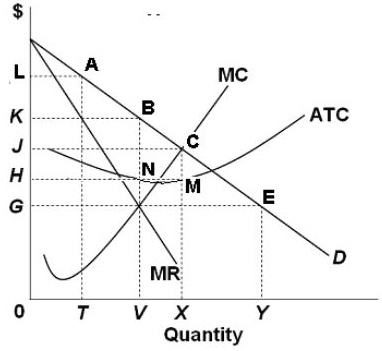
MULTIPLE CHOICE: Use the graph above. The
maximum profits for this monopolist can be represented by which area
on the graph?
1. 0KBD
2. 0HCX
3. HKBN
4. 0HNV
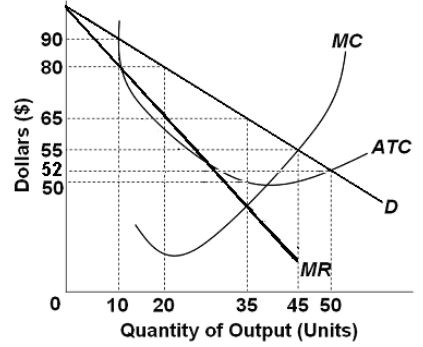
MULTIPLE CHOICE: Use the graph above. What
are the profits earned by this monopolist at the profit maximizing
level of output?
1. $ 2275
2. $ 1750
3. $ 4275
4. $ 525
Find the profit maximizing quantity,
price, and profits, using the table of data below.
Demand Data
Cost
Data
Quantity
PriceDemanded
Output
Total Cost
$5.5033$5.00
5.0044
6.00
4.5055
6.50
3.8566
7.50
3.3577
9.00
2.908811.00
2.509914.00
Monopoly: Short Run Earning
Profits
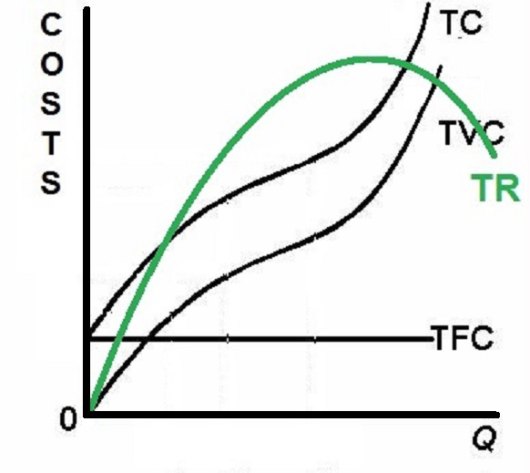
Monopoly: Short Run Earning
Losses
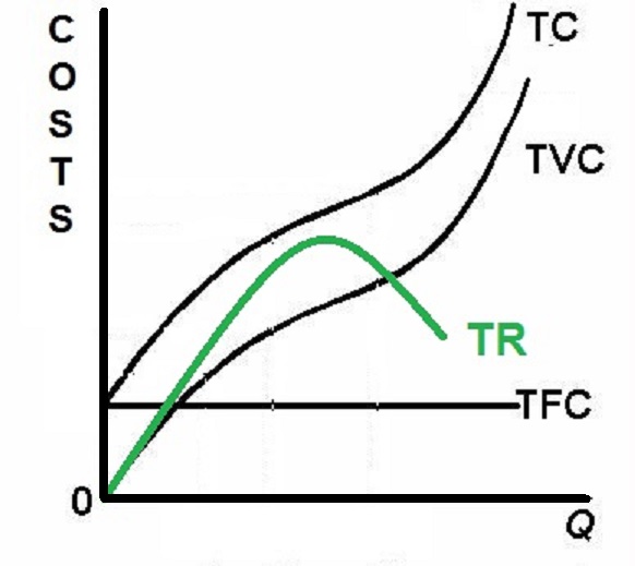
Monopoly: Short Run Shut
Down
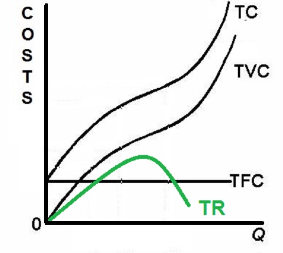
- Micro
4.1 Monopoly Demand and MR: Econ Concepts in 60 Seconds monopoly
graph
[4:41 YouTube ACDC Leadership]
NOTE: These are REVIEW videos only. In order to
learn the material you must read the assigned textbook readings,
watch the assigned lecture videos, and do problems. See the
MICWEBAPP
or the LESSONS
link for these assignments.
Unit 3: Are Businesses Efficient?
Product Markets and Efficiency
Lesson 10b: Monopoly: Long Run
Equilibrium:
Efficiency, Price Discrimination, and Regulation
ARE BUSINESSES EFFICIENT?
In lesson 8/9b we learned that in the long run
purely competitive firms are both allocatively and productively
efficient. They maximize society's satisfacton. In lesson 10a we
learned how to find the quantity produced by monopolies. Here in
lesson 10b we will learn if that quantity that we get, the profit
maximiing quantity, is the efficient quantity that we want. Are
monopolies efficient? Are businesses efficient?
In lesson 8/9b we also learned that if purely
competitive firms have short run profits, then in the long run new
firms will enter. This will increase the supply of the product
because if the number of producers increases then supply increases
(lesson 3b). When supply increases it causes the price to drop and
this will reduce the profits of the firms. This will continue to
happen until there are just normal profits. In the long run, purely
competitive firms earn only normal (zero) profits BECAUSE THERE ARE
NO BARRIERS TO ENTRY.
So, what about monopolies? In this lesson we
will learn that SINCE MONOPOLIES DO HAVE BARRIERS TO ENRTY (entry is
blocked) they will earn economic profits in the long run.
Also, at the profit maximizing quantity (what we get) monopolies will
be both allocatively and productively INEFFICIENT. When monopolies
produce the quantity that maximizes their profits they will be
producing less than the allocatively efficient quantity
(underallocation of resources) AND they will not be producing at the
lowest possible cost per unit (productive inefficiency).
Next, we will look at PRICE DISCRIMINATION.
What if instead of charging the same price to all customers, a
monopoly charged different prices to different customers for the same
product? We will learn that if monopolies price discriminate then
they will produce more, and the market will be MORE allocatively
efficient.
Finally, since monopolies are inefficient, the
government usually prevents them from forming (anti-trust laws).
Sometimes the government will allow a monopoly to exist if it is in
the public interest, like when it is a natural monopoly, but they
will then regulate it, i.e. set its price.
So in this lesson we will study three
things:
1. monopolies are allocatively and
productively inefficient
2. monopolies that price discriminate may be allocatively
efficient
3. monopolies are often prevented from forming or are broken up by
the government, but the government will allow a natural monopoly
to exist and will regulate its price.
10b Something Interesting - Why are
we studying this?
|
Why do state governments prevent competition
in the distribution of electricity? In northern Illinois only ComEd
can run electricity wires from house to house.
- ANSWER: The distribution of
electricity is a natural monopoly. It is productively
more efficient to have only one company running wires from
house to house. With fewer wires we can get the same amount of
elctricity. So, the government only gives a license to one company
to distribute electricity because it saves resources compared to
having several companies distribute electricity in the same
neighborhood.
Once the government creates a monopoly like
ComEd, why will they then regulate the price of electricity? In
Illinois the state run Illinois Commerce Commission sets the price of
electricity.
- ANSWER: In this lesson we will learn
that monopolies are allocatively inefficient. They will
charge a high price and sell less to maximize profits. This is bad
for society so the goverment regulates the price.
10b Assignments: Readings
|
pp. 263-273, (19th, 203-214), "Economic Effects
of Monopoly", "Price Discrimination", "Regulated Monopoly"
pp. 431-438, (19th, 376-384), "Antitrust
Policy: Issues and Impacts", "Industrial Regulation"
pp. 146-147, (19th, 86-87), "Last Word -
Elasticity and Pricing Power: Why Different Consumers Pay Different
Prices"
Lecture
Outline
10b Assignments: Video
Lectures
|
THE SOCIAL COST OF MONOPOLY
6.2.1 Determining
the Social Cost of Monopoly 12:22
[MyNotes]
6.2.2
Calculating
Deadweight Loss 15:23
[MyNotes]
PRICE
DISCRIMINATION
Price
Discrimination and its Effects on Efficiency in a Monopolistic
Market (econclassroom.com)
14:51
REGULATING
NATURAL MONOPOLIES
Natural
Monopoly and the Need for Government
Regulation (econclassroom.com)
14:14
10b Outcomes - What you should
learn
|
TOPICS
- Long Run Equilibrium
- Monopolies and Efficiency
(Inefficient)
- Price Discrimination
- Natural Monopolies and
Regulation
OUTCOMES
- Discuss the economic effects of pure
monopoly on price, quantity produced, allocative efficiency,
productive efficiency, dynamic efficiency (technological
progress), X-efficiency, and distribution of income
(equity).
- Understand the adjustment process from the
short run to the long run and the role of barriers to
entry. Why does a monopoly earn economic
profits in the long run?
- Draw the long run equilibrium graph for a
pure monopoly and indicate the profit maximizing quantity, the
allocatively efficient quantity, and the productively efficient
quantity.
- Define price discrimination, list three
conditions necessary for price discrimination, explain how price
discrimination affects allocative efficiency, explain why profits
and output will be higher for a discriminating
monopoly.
- Identify two pricing strategies of monopoly
regulation and explain the dilemma the regulators face in
utilizing these strategies
- Explain why a regulated monopoly may not
have an incentive to reduce costs.
- Why does the Illinois government allow
ComEd to have a monopoly on the distribution of electricity in
northern Illinois?
Key Terms
Flash Cards - Click Here
Key Terms:
allocative inefficiency, productive
inefficiency, deadweight loss, economies of scale, natural
monopoly, X-inefficiency, dynamic efficiency, anti-trust policy,
price fixing, tying contract, public interest theory of
regulation, legal cartel theory of regulation, deregulation, price
discrimination, regulated monopoly, natural monopoly,
socially-optimal price (allocatively efficient price), fair-return
price (average-cost price)
Monopoly
- Long Run Equilibrium and Efficiency - Click Here
Price
Discrimination - How to find the profit maximizing quantity on a
table - Click Here
[works for me if I save the file to my computer first, then open
it]
Monopoly - Long Run Equilibrium and
Efficiency
Explain why Monopolies earn economic
profits in the long run
Draw the long run equilibrium graph for a
Monopoly
Explain why Monopolies are inefficient in
the long run and show the following on the graph:
- the profit maximizing
quantity
- the allocatively efficient quantity
- the productively efficient quantity
Price Discrimination - How to find the
profit maximizing quantity on a table
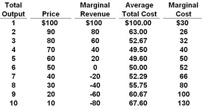
MULTIPLE CHOICE:
10. Refer to the above data for a
nondiscriminating monopolist. This firm will maximize
its profit by producing what quantity?
A. 3 units
B. 4 units
C. 5 units
D. 6 units
11. If the above data was for a PERFECTLY PRICE
DISCRIMINATING MONOPOLIST it would maximize its profit by producing
what quantity?
A. 3 units
B. 4 units
C. 5 units
D. 6 units
12. If the above data was for a PERFECTLY PRICE
DISCRIMINATING MONOPOLIST what would its total revenue be at the
profit maximizing quantity?
A. $ 60
B. $ 300
C. $ 400
D. zero
13. If the above data was for a PERFECTLY PRICE
DISCRIMINATING MONOPOLIST what would its profit be at the profit
maximizing quantity?
A. zero
B. $ 152
C. $ 248
D. $ 400
Monopoly: Long Run
Equilibrium
- M is the profit maximizing quantity
(MR=MC); What We Get
- Q is the allocatively efficient quantity (P=MC); What We
Want
- N is the productively efficient quantity (MC=ATC); producing at
a minimum cost
Regulated Natural
Monopoly
- Q3 is the profit maximizing quantity
(MR=MC) if unregulated
- Q2 is the allocatively efficient quantity (P=MC)
- Q4 is the productively efficient quantity (MC=ATC)
- Q1 is the "fair return" quantity if regulated
Monopoly with Perfect Price
Discrimination
- M is the profit maximizing quantity
(MR=MC) if no price discrimination; What We Get
- Q is the profit maximizing quantity (D=MR=MC) if there is
perfect price discrimination
- Q is also the allocatively efficient quantity (P=MC); What We
Want
- N is the productively efficient quantity (MC=ATC); Producing at
a Minimum Cost
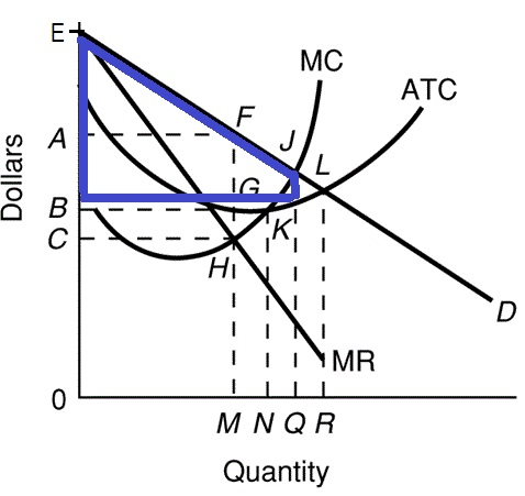
- Monopoly
Graph Review and Practice- Micro 4.7
[5:34 YouTube ACDC Leadership]
- Micro
4.8 Price Discriminating Monopoly (First
Degree)
[4:41 YouTube ACDC Leadership]
NOTE: These are REVIEW videos only. In order to
learn the material you must read the assigned textbook readings,
watch the assigned lecture videos, and do problems. See the
MICWEBAPP
or the LESSONS
link for these assignments.
Unit 3: Are Businesses Efficient?
Product Markets and Efficiency
Lesson 11a: Monopolistic Competition:
Are Businesses Efficient?
ARE BUSINESSES EFFICIENT?
Competitive firms are efficient and monopolies
are inefficient, but there are few if any purely competitive markets
or purely monopolistic markets (monopolies). So what happens in the
real world? Are businesses efficient?
We learned that competitive firms earn
zero long run profits because there are no barriers to entry and
monopolies do earn long run profits because entry is blocked.
What about monopolistically competitive markets where there are LOW
BARRIERS? What about oligopolistic markets where there are HIGH
BARRIERS? Guess what? If there are low barriers firms will earn zero
long run profits (monopolistic competition) and if there are high
barriers firms will earn long run economic profits
(oligopolies).
What about efficiency? We will learn that both
monopolistically competitive firms and oligopolies are inefficient
but not to the same degree. Monopolistically competitive firms are
only slightly inefficient and they do provide society some additional
benefits, but oligopolies can be very inefficient and are closely
watched by the government.
General Outline for Each Product Market
Model:
1. Know the model's characteristics
and examples (See the "8/9a QUIZ - 4 PRODUCT MARKETS" quiz on our
Blackboard site.)
2. Be able to explain the shape of the demand curve
3. Draw the short run equilibrium graphs for (a) profit maximizing
firms, (b) loss minimizing firms, and (c) firms that will shut
down
4. Draw the long run equilibrium graph and find the profit
maximizing quantity (WHAT WE GET), allocatively efficient quantity
(WHAT WE WANT), and the productively efficient quantity. See the
last 13 pages of the Unit 3 Yellow Pages ("3 Rules and 4
Models").
5. Understand any other issues associated with the model
Never forget this: To maximize profits
businesses will produce the quantity where MR=MC.
11a Something Interesting - Why are
we studying this?
|
Why are there so many different kinds of
hamburgers?
Wikipedia has a list of over 30 different types
of hamburgers [https://en.wikipedia.org/wiki/List_of_hamburgers].
Why are there so many? Why do different restaurants continue to
invent their own "new" hamburger?
ANSWER: In this lesson you will learn that
firms gain market power through product differentiation
- making their product a little different from their competitors.
This allows them to charge a higher price and increase their profits.
BUT, other restaurants can always copy the new hamburger recipe
stealing away those profits. Welcome to Monopolistic Competition:
part "monopoly" because of product differentiation and part "pure
competition" because of low bariers to entry.
11a Assignments: Readings
|
pp. 278-286, (19th, 216-223), "Monopolistic
Competition", "Price and Output in Monopolistic Competition",
"Monopolistic Competition and Efficiency", "Product
Variety"
Lecture
Outline
11a Assignments: Video
Lectures
|
6.4.1 Defining
Monopolistic Competition 7:01
[MyNotes]
6.4.2
Understanding
Pricing and Output in Monopolistic Competition
- Short-Run Profit Maximization for a Monopolistically Competitive
Firm - 8:58 [MyNotes]
Monopolistic
Competition (econclassroom.com --
efficiency begins at 15:00) 20:51
Monopolistic
Competition in the Long-Run: Econ Concepts in 60 Seconds with AP
Economics Teacher (ACDCEcon)
3:25
11a Outcomes - What you should
learn
|
TOPICS
- Characteristics and Examples of
Monopolistic Competition
- Short Run Equilibrium
- Long Run Equilibrium and
Efficiency
OUTCOMES
- List the characteristics of monopolistic
competition.
- How many is “many”?
(Concentration Ratio and Herfindahl Index)
- Explain how product differentiation occurs
in similar products.
- Determine the profit maximizing price and
output level for a monopolistic competitor in the short run when
given cost and demand data.
- Explain why a monopolistic competitor will
realize only normal profit in the long run.
- Draw the short run equilibrium graphs for a
monopolistically competitive firm that (a) maximizes profit, (b)
minimizes loss, and (c) shuts down
- Understand the adjustment process from the
short run to the long run and the role of barriers to entry (why
do monopolistically competitive firms earn zero economic profits
in the long run?)
- Draw the long run equilibrium graph for a
monopolistically competitive firm and indicate the profit
maximizing quantity, the allocatively efficient quantity, and the
productively efficient quantity.
- Why does a monopolistically competitive
firm earn zero economic profits (normal profits) in the long
run?
- Identify the reasons for excess capacity in
monopolistic competition.
- Explain how product differentiation may
offset the inefficiency of monopolistic competition.
Key
Terms Flash Cards - Click Here
Key Terms:
monopolistic competition, product
differentiation, collusion, nonprice competition, four-firm
concentration ratio, Herfindahl index, normal profit, excess
capacity
Monopolistic
Competition - How to find the quantity, price, and profit on a graph
- Click Here
[works for me if I save the file to my computer first, then open
it]
Monopoly
- Long Run Equilibrium and Efficiency - Click Here
Monopolistic Competition - How to find
the quantity, price, and profit on a graph
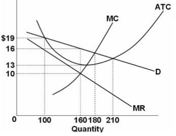
3.MULTIPLE CHOICE: Refer to the above
diagram for a monopolistically competitive firm in short-run
equilibrium. This firm will realize an economic:
A. loss of $320
B. profit of $480
C. profit of $280
D. profit of $600
Monopolistic Competition - Long Run
Equilibrium and Efficiency
Explain why Monopolistically
Competitive firms earn zero economic profits in the long
run
Draw the long run equilibrium graph for
Monopolistic Competition
Discuss the efficiency of Monopolistically
Competitive firms in the long run and show the following on the
graph:
- the profit maximizing
quantity
- the allocatively efficient quantity
- the productively efficient quantity
Herfindahl index =  MARKET SHARE SQUARED
HI =
ms12 + ms22 +
ms32 + ms42 +
ms52 + .. . . .
"
"means "sum" or "add all together"
"ms" means "% market share"
Monopolistic Competition in Short Run
Equilibrium
Monopolistic Competition in Long Run
Equilibrium
- D is the profit maximizing quantity
(MR=MC); What We Get
- G is the allocatively efficient quantity (P=MC); What We
Want
- E is the productively efficient quantity (MC=ATC): Produce at a
Minimum Cost
Monopolistic
Competition- Short Run and Long Run- Micro
4.12
[2:02 YouTube ACDC Leadership]
NOTE: These are REVIEW videos only. In order to
learn the material you must read the assigned textbook readings,
watch the assigned lecture videos, and do problems. See the
MICWEBAPP
or the LESSONS
link for these assignments.
Unit 3: Are Businesses Efficient?
Product Markets and Efficiency
Lesson 11b: Oligopoly: Are Businesses
Efficient?
ARE BUSINESSES EFFICIENT?
Oligopolies are industries with just a few
firms because there are high barriers to entry. So do they earn
long-run profits (YES) and are they efficient (NO)?
Oligopolies are more complex than the other
three models. Instead of one model to explain how oligopolies
determine price and quantity we will have four:
1. kinked demand model
2. collusion
3. price leadership
4. game theory
General Outline for Each Product Market
Model:
1. Know the model's characteristics
and examples (See the "8/9a QUIZ - 4 PRODUCT MARKETS" quiz on our
Blackboard site.)
2. Be able to explain the shape of the demand curve
3. Draw the short run equilibrium graphs for (a) profit maximizing
firms, (b) loss minimizing firms, and (c) firms that will shut
down
4. Draw the long run equilibrium graph and find the profit
maximizing quantity (WHAT WE GET), allocatively efficient quantity
(WHAT WE WANT), and the productively efficient quantity. See the
last 13 pages of the Unit 3 Yellow Pages ("3 Rules and 4
Models").
5. Understand any other issues associated with the model
Never forget this: To maximize profits
business will produce the quantity where MR=MC.
11b Something Interesting - Why are
we studying this?
|
Are these mergers good for society? How do they
affect efficiency? Just skim the first few paragraphs of the
following:
- The
T-Mobile-Sprint Merger: The End Is Near
(2019)
- Airline
Mergers Push Fares Higher
(2013)
- Beer
merger will not bring Budweiser, Miller under same
roof (2015)
- U.S.
Justice Department urges judge to block AT&T-Time Warner
merger (2018)
ANSWER: It is often up to the US Justice
Department to determine whether or not to allow businesses to merge
into one single business. Such mergers can reduce competition, raise
prices, and cause allocative and productive inefficiency. "Their job,
essentially, is to figure out whether a merger would reduce
competition so much that a company could raise prices without losing
business to competitors."
11b Assignments: Readings
|
pp. 286-299, (19th, 223-240), "Oligopoly",
"Oligopoly Behavior: A Game-Theory Overview", "Three Oligopoly
Models", "Oligopoly and Advertising", "Oligopoly and Efficiency",
"Last Word - Internet Oligopolies"
pp. 304-309, (19th, 241-242), "Additional Game
Theory Applications"
pp. 433-434, (19th, 379-380),
"Mergers"
Lecture
Outline
11b Assignments: Video
Lectures
|
OLIGOPOLY
Game Theory
EconMovies
8: The Dark Knight (Oligopolies and Game
Theory) 7:01
6.3.1
Introducing
Oligopoly and the Prisoner's Dilemma
17:26 [MyNotes]
6.4.3
Understanding
Monopolistic Competition (Oligopoly ???) as a Prisoner's
Dilemma - Advertising and Brand Names
6:44 [MyNotes]
6.3.2
Understanding
a Cartel as a Prisoner's Dilemma
10:47 [MyNotes]
Kinked
Demand Model
6.3.3 Understanding
the Kinked-Demand Curve Model
4:22 [MyNotes]
Kinked
Demand Model of Oligopoly Pricing
(econclassroom.com) 14:06
Other
Oligopolies,
Duopolies, Collusion, and Cartels
(Khan Academy) 8:26
Episode
30C: Mergers (YouTube: mjmfoodle)
4:36
SUMMARY
Determining
the Efficiency of Firms in Different Market
Structures (econclassroom.com)
18:23
11b Outcomes - What you should
learn
|
TOPICS
- oligopoly
- mergers
- game theory
OUTCOMES
- Describe the characteristics of an
oligopolistic industry.
- Differentiate between homogeneous and
differentiated oligopolies.
- Describe and compare the concentration
ratio and the Herfindahl index as ways to measure market dominance
in an industry.
- Distinguish between three types of
mergers.
- Explain how the Herfindahl index is used as
a guideline by the government in deciding whether to permit
horizontal mergers.
- Use a profit-payoffs matrix (game theory)
to explain the mutual interdependence of two rival firms and why
oligopolists might tempt to cheat on a collusive
agreement.
- Identify four possible models of
oligopolistic price-output behavior.
- Use the kinked demand curve theory to
explain why prices tend to be inflexible.
- Why is there a "kink" in the kinked demand
curve?
- Understand the adjustment process from the
short run to the long run and the role of barriers to entry (why
do oligopolistic firms earn economic profits in the long
run?)
- Draw the long run equilibrium graph for a
kinked demand oligopoly and indicate the profit maximizing
quantity, the allocatively efficient quantity, and the
productively efficient quantity.
- Explain the major advantages of collusion
for oligopolistic producers and list the obstacles to collusive
behavior.
- Draw the long run equilibrium graph for a
collusive oligopoly and indicate the profit maximizing quantity,
the allocatively efficient quantity, and the productively
efficient quantity. (Hint: it is just like the long run monopoly
graph.)
- Explain price leadership as a form of tacit
collusion.
- List the positive and negative effects of
advertising.
- Explain why some economists assert that
oligopoly is less desirable than pure monopoly.
- Are these mergers good for society
(efficiency)?
Key
Terms Flash Cards - Click Here
Key Terms:
oligopoly, homogeneous (standardized)
oligopoly, differentiated oligopoly, mutual interdependence,
interindustry competition, collusion, kinked demand, cartel, price
leadership, merger, horizontal merger, vertical merger,
conglomerate merger, game theory, strategic behavior, prisoner's
dilemma, dominant strategy, Nash equilibrium, self enforcing
agreement
Oligopoly:
The Kinked Demand Model - Click Here
Oligopoly
- Long Run Equilibrium and Efficiency - Click Here
Oligopoly: The Kinked Demand
Model
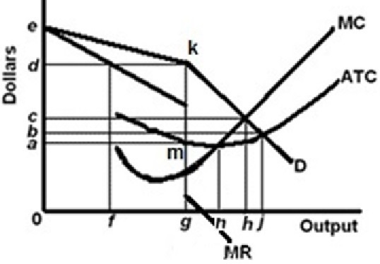
What are the assumptions behind the
model?
Why is the demand kinked (bent)?
Use the graph above to find:
- the profit maximizing price and
quantity
- the long run profits
- the allocatively efficient Q
- the productively efficient Q
How does the model show price
inflexibility?
What are the criticisms of the model?
Oligopoly - Long Run Equilibrium and
Efficiency
Explain why Oligopolies earn economic
profits in the long run
Draw the long run equilibrium graph for a
Kinked Demand Oligopoly
Discuss the efficiency of Oligopolies in the
long run and show the following on the kinked demand
graph:
- the profit maximizing
quantity
- the allocatively efficient quantity
- the productively efficient quantity
Oligopoly Kinked Demand Long Run
Equilibrium
- 10 is the profit maximizing quantity
(MR=MC) What We Get
- 14 is the allocatively efficient quantity (P=MC); What We
Want
Oligopoly Game Theory
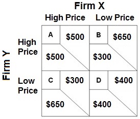
Micro
4.11 Kinked Demand Curve: Econ Concepts in 60 Seconds
[2:02 YouTube ACDC Leadership]
Micro
4.9 Oligopolies and Game Theory: Microeconomics Concepts in 60
Seconds with Mr. Clifford
[3:24 YouTube ACDC Leadership]
NOTE: These are REVIEW videos only. In order to
learn the material you must read the assigned textbook readings,
watch the assigned lecture videos, and do problems. See the
MICWEBAPP
or the LESSONS
link for these assignments.
Unit 4: Labor and Efficiency: Resource
Markets, Inequality, and Immigration
Lesson 12a: Demand For
Resources
In unit 3 we studied the FOUR PRODUCT
MARKET MODELS to learn how product prices and quantity are
determined. We learned characteristics and examples of each model. We
discussed the differences between their demand curves. We drew their
short run equilibrium graphs and found the long run equilibrium
quantity, allocatively efficient quantity, and the productively
efficient quantity. Finally we discussed other issues associated with
some of the models.
In unit 4 we will discuss the TEN LABOR
(or resource) MARKET MODELS to learn how wages and the level of
employment are determined. We will learn what determines how much
people will be paid and how many people will be hired, i.e. the
profit maximizing quantity to hire. Then we will determine
whether businesses hire the allocatively efficient quantity of
labor.
We will finish the unit by looking at two
important issues associated with labor markets: income inequality and
immigration.
This lesson begins our study of the labor
markets by looking at the demand for resources, the elasticity of
demand for resources, and the first two labor market models: (1) a
competitive labor market working in a competitive product market, and
(2) a competitive labor market working in an imperfectly competitive
product market (like a monopoly or oligopoly). We will find the
profit maximizing quantity of labor (and wage) that will be hired and
the allocatively efficient quantity of labor that would maximize
society's satisfaction
We will use benefit-cost analysis (BCA)
throughout this unit. It would be useful to review BCA in lesson 1d.
For example, to find the profit maximizing quantity of workers to
hire firms will continue to hire up to the point where MRP =
MRC.
12a Something Interesting - Why are
we studying this?
|
Look at the websites below.
Lowest Paying College Majors:
http://money.cnn.com/2015/05/08/pf/college/lowest-paying-college-majors/index.html
Highest Paying College Majors:
http://money.cnn.com/2015/05/07/pf/college/highest-paying-college-majors/index.html
Why are people paid differently?
ANSWER: The supply and demand for labor helps
explain why different people and different jobs receive different
wages. But there are also other factors that we will need to explore.
We will end up with 8 to 10 different labor market models that will
help us answer this question.
12a Assignments: Readings
|
pp. 312-321, 322-324, (19th, 248-257, 260-261),
"Significance of Resource Pricing", "Marginal Productivity Theory of
Resource Demand", "Determinants of Resource Demand", "Elasticity of
Resource Demand", "The Profit-Maximizing Rule", NOT "The Least Cost
Rule"
Lecture
Outline
12a Assignments: Video
Lectures
|
7.1.1 Deriving
the Factor Demand Curve 15:10
[MyNotes]
7.1.3 Analyzing
the Labor Market 15:24
[MyNotes]
(THE
LOST EPISODES) Factor Market Overview
(YouTube mjmfoodle) 1:27
(The
Lost Episodes) Perfectly Competitive Factor and Output
Markets (YouTube mjmfoodle)
5:14
5.2
Perfectly Competitive Labor Market and Firm: Econ Concepts in 60
Seconds (YouTube ACDC Econ)
3:27
Micro
5.3 Comparing Product and Resource Markets: Econ Concepts in 60
Seconds- Review (YouTube ACDC Econ)
2:24
OPTIONAL Snow Day Lecture - During the
2018-2019 school year we had a snow day when lesson 12a was scheduled
in our on-campus class. To avoid losing a day of class I recorded the
lesson 12a lecture and posted it online. Here it is: Lesson
12a Snow Day lecture (1hour 15
minutes)
12a Outcomes - What you should
learn
|
TOPICS
- Finding the Resource Demand
Curve
- Determinants of Resource Demand
- Elasticity of Resource Demand
- The Profit Maximizing Quantity to
Hire:
- The Allocatively Efficient Quantity to
Hire:
- The First Two Labor Market Models:
- Competitive labor market in a
competitive product market
- Competitive labor market in an
imperfecly comp. prod. market
OUTCOMES
- Why is resource demand a "derived
demand?
- List the three determinants of demand for a
resource and explain how a change in each of the determinants
would affect the demand for the resource.
- List three determinants of the price
elasticity of demand for a resource, and state how changes in each
would affect the elasticity of demand for a resource.
- Describe a competitive labor
market
- Define and calculate the
marginal-revenue-product (MRP). Explain why the MRP schedule of a
resource is the firm's demand schedule for the resource in a
purely competitive product market. Explain
why the resource demand curve is downward sloping. DEFINE, DRAW,
DESCRIBE.
- For a competitive labor market use
benefit-cost analysis (the MRP = MRC principle) to find the
profit maximizing quantity of labor a firm will employ in a
purely competitive product market and in an imperfectly
competitive product market when given the data and
graph.
- For a competitive labor market use
benefit-cost analysis (VMP = W) to find the allocatively
efficient quantity of labor for a firm to employ in a purely
competitive product market and in an imperfectly competitive
product market when given the data and graph.
12a Determinants of Labor Demand and
Elasticity of Labor Demand
|
DETERMINANTS OF LABOR DEMAND
1. Changes in Demand for the Product (derived
demand)
- If demand for the product increases then
demand for labor used to make that product will
increase
- If demand for the product decreases then
demand for labor used to make that product will
decrease
2. Productivity Changes
- If the productivity of labor increases then
demand for labor will increase
- If the productivity of labor decreases then
demand for labor will decrease
-
Factors that affect the productivity of Labor:
- the quantity of nonlabor inputs
used: more other resources used with labor = more
productivity of labor
- technological progress: more
technological progress = more productivity of
labor
- labor quality: better quality =
more productivity
3. Changes in the Prices of Other Resources
(Substitutes and Complements)
- Substitute Resources
- Substitution effect
- an increase in price of a substitute
resource will cause the demand for labor to
increase
- a decrease in the price of a
substitute resource will cause the demand for labor to
decrease
- Output effect
- an increase in price of a substitute
resource will cause the quantity of product produced to
decrease and the demand for labor will decrease
- a decrease in price of a substitute
resource will cause the quantity of product produced to
increase and the demand for labor will increase
- Net effect
- if the substitution effect is greater
than the output effect then a decrease in the price of a
substitute resource will decrease the demand for
labor
- if the output effect ois greater than
the substitution effect then a decrease in the price of a
substitute resource will increase the demand for
labor
- Complementary Resources
- an increase in price of a complementary
resource will cause the demand for labor to
decrease
- a decrease in the price of a
complementary resource will cause the demand for labor to
increase
DETERMINANTS OF THE ELASTICITY OF LABOR
DEMAND
1. Ease of Resource Substitutability
- the greater the number of substitute
resources, then the demand for labor is lmore elastic
- the fewer the number of substitute
resources, then the demand for labor is less elastic
2. Elasticity of Product Demand
- the more elastic the demand for the
product, then the demand for labor used to produce that product is
more elastic
- the less elastic the demand for the
product, then the demand for labor used to produce that product is
less elastic
3. Labor-Cost to Total-Cost Ratio
- if labor is a greater proportion of the
total costs of production, then the demand for labor is more
elastic
- if labor is a smaller proportion of the
total costs of production, then the demand for labor is less
elastic
Key Terms
Flash Cards - Click Here
Key Terms:
derived demand, productivity, marginal
product (MP), marginal revenue product (MRP), marginal resource
cost (MRC), profit maximizing rule for hiring resources (MRP=MRC
rule), value of the marginal product (VMP), substitute resources,
complementary resources, substitution effect, output effect,
elasticity of resource demand, marginal productivity theory of
income distribution
Finding the Quantity to Hire: Competitive Labor
Market in a Competitive Product Market
Finding the Quantity to Hire: Competitive Labor
Market in an Imperfectly Competitive Product Market
Competitive Labor Market in a Competitive
Product Market -
Problem 1
Answer the questions below on the
basis of the information given in the following table.
The labor market is competitive where the wage rate is $10.
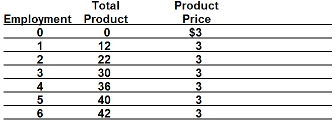
Refer to the above data. How can you tell
that this firm is selling its product in a purely competitive
product market?
MULTIPLE CHOICE: Refer to the above data. If
the firm is hiring workers under purely competitive conditions at
a wage rate of $10, it will employ:
A. 2 workers
B. 3 workers
C. 4 workers
D. 5 workers
Refer to the above data. What is the labor
demand schedule for this firm?
Refer to the above data. What is the
allocatively efficient quantity to hire?
Competitive Labor Market in a Competitive
Product Market -
Problem 2
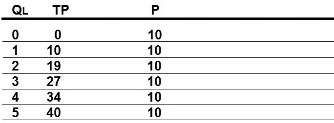
Use the data above to calculate: (1) the
quantity of labor that this firm will hire to maximize profits,
and (2) the allocatively efficient quantity to hire.
Assume the firms hires labor, its only
variable input, under competitive conditions at a wage rate of $70
and sells its products under competitive conditions for a price of
$10.
Competitive Labor Market in an
Imperfectly Competitive Product Market - Problem 1
Answer this questions below on the
basis of the information given in the following table.
The labor market is competitive where the wage rate is $10.
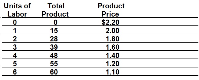
Refer to the above data. How can you tell
that this firm is selling its product in an imperfectly
competitive product market like a monoploy, oligopoly, or
monopolistic competition?
MULTIPLE CHOICE: Refer to the above data. If
the firm is hiring workers under purely competitive conditions at
a wage rate of $10, it will employ:
A. 2 workers
B. 3 workers
C. 4 workers
D. 5 workers
Refer to the above data. What is the
allocatively efficient quantity to hire?
Competitive Labor Market in an
Imperfectly Competitive Product Market - Problem 2

Use the data above to calculate: (1)
the quantity of labor that this firm will hire to maximize
profits, and (2) the allocatively efficient quantity to
hire.
Assume the firms hires labor, its only
variable input, under competitive conditions at a wage rate of $70
and sells its products under imperfectly competitive (monopoly)
conditions at the prices listed.
marginal product: MP = TP
/ Qres
marginal revenue product: MRP = TR
/ Qres
marginal resource cost: MRC = TC
/ Qres
profit maximizing rule for hiring resources:
MRP=MRC
value of the marginal product: VMP = P x
MP
allocative efficiency quantity of resources:
VMP = W
Circular Flow Model: 4 Product Market
Models and 8 (10) Labor Market Models
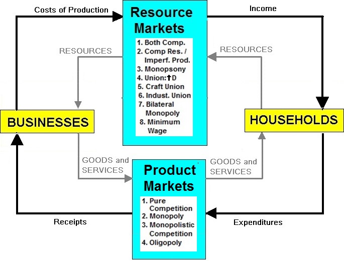
Competitive Labor Market in a Competitive
Product Market
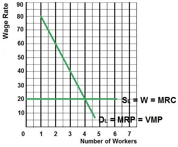
Competitive Labor Market in an
Imperfectly Competitive Product Market
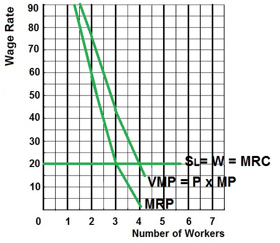
- 5.2
Perfectly Competitive Labor Market and Firm: Econ Concepts in 60
Seconds- Advanced Placement
[3:29 YouTube ACDC Leadership]
- Micro
5.3 Comparing Product and Resource Markets: Econ Concepts in 60
Seconds- Review
[2:27 YouTube ACDC Leadership]
-
Micro 5.4 Resource Market, MRP and MRC: Econ Concepts in 60 Seconds-
Factor Market
[2:54 YouTube ACDC Leadership]
NOTE: Mr Clifford says "MRP = P x MP" This is true ONLY IF we have a
competitive labor market (wage is constant). I prefer to use the
formula: "MRP = change in TR / change in Qlabor", because this works
for ALL labor market models
NOTE: These are REVIEW videos only. In order to
learn the material you must read the assigned textbook readings,
watch the assigned lecture videos, and do problems. See the
MICWEBAPP
or the LESSONS
link for these assignments.
Unit 4: Labor and Efficiency: Resource
Markets, Inequality, and Immigration
Lesson 13a: Wage Determination: Labor
Markets
Ten Labor Market Models
1. Competitive labor market in a
competitive product market
2. Competitive labor market in an imperfectly competitive product
market
3. Monopsony
4. Union Model: increasing demand for labor
5. Union Model: craft (exclusive) union
6. Union Model: industrial (inclusive) union
7. Union Model: bilateral monopoly
8. Minimum Wage (three models)
a. traditional minimum wage model
(price floor)
b. minimum wage in a monopsony
c. minimum wage and the price elasticity of demand for
labor
For EACH model know the
following:
1. assumptions, characteristics, and
examples
2. graph
3. find the profit maximizing quantity of labor (this is the
quantity that WILL BE HIRED, where MRP = MRC)
4. find the allocatively efficient quantity of labor (where VMP =
W or Qd=Qs)
You will find a summary of each of these ten
models in our YELLOW PAGES, on the LESSONS webpage, and on the
MICWEBAPP. It is strongly recommended that you study these
summaries.
REMEMBER: to find the profit maximizing
quantity of workers to hire firms will continue to hire up to the
point where MRP = MRC.
So for any questions that ask "how many will
be hired?" or "what will the wage be?", the first thing you do is
calculate MRP and MRC and then hire all where the MRP is greater than
MRC (MRP > MRC) up to where MRP = MRC.
13a Something Interesting - Why are
we studying this?
|
What if the federal miniumum wage doubled to
$15 an hour. Would this help or hurt fast food workers?
ANSWER: After studying this lesson you should
be able to explain the following statement found in this news
report:
http://www.marketplace.org/topics/wealth-poverty/fast-food-strike-walk-outs-and-drive-throughs
" . . . if we woke up tomorrow and
fast food restaurants had doubled worker pay tomorrow . . . I'm
sure you would see a lot of jobs lost , . . . But that’s only
part of the story, Baker argues. Even if there was, let’s
say, a 20 or 30 percent drop in employment at these places
(Saltsman told me he projects there could be up to a 27 percent
drop), the remaining workers would still “take home twice as
much pay. They're still way better off,” says Baker."
To understand and explain this statement you
need to discuss price elasticity of demand for workers. Does Baker
think that the price elasticity of demand for fast food workers is
elastic or inelastic? [Answer: Inelastic]
13a Assignments: Readings
|
330-351, (19th, Ch. 13, ALL)
Summary
of the 8 Labor Market Models (The last
17 pages of the Unit 4 Yellow Pages)
Audio: Fast
food strike: Of walk outs and drive-throughs
Economists
disagree on whether the minimum wage kills jobs. Why?
Interesting: "Minimum
Wage Would Be $21.72 If It Kept Pace With Increases In Productivity:
Study"
Lecture
Outline
13a Assignments: Video
Lectures
|
(THE
LOST EPISODES) Monopsony Factor Market, Perfectly Competitive Output
Market (YouTube mjmfoodle
8:11)
Micro
5.1 Market and Minimum Wage: Econ Concepts in 60 Seconds:- Economics
Lesson (YouTube ACDC Econ
3:26)
11.4.2
An
Analysis of Labor Unions and Unemployment
(7:27) [MyNotes]
11.4.1
Minimum
Wage Laws (7:31) [MyNotes]
11.4.4 The
Theory of Efficiency Wages (10:54)
[MyNotes]
OPTIONAL: 11.4.3 Something
Interesting: "La Causa": The United Farm
Workers (5:10) MyNotes]
13a Outcomes - What you should
learn
|
TOPICS
- Wages and Productivity
- 8 labor market models
- Why wages differ
OUTCOMES
- List those factors that have led to an
increasing level of labor productivity and real wages in the
U.S.
- Describe the following labor market models.
Determine the equilibrium wage rate, employment level, and its
effect on efficiency. Be able to Define, Draw, and Describe the
shapes of the graphs for each model.
- Competitive labor market in a
competitive product market (table of data and a
graph)
- Competitive labor market in an
imperfectly competitive product market (table of data and a
graph)
- Monopsony (table of data and a
graph)
- Union Model: increasing demand for
labor
- Union Model: craft (exclusive)
union
- Union Model: industrial (inclusive)
union
- Union Model: bilateral
monopoly
- Minimum Wage Models
- traditional minimum wage
model
- minimum wage in a
monopsony
- minimum wage and the price elasticity
of demand for labor
- Why wages differ - Explain the demand and
supply factors that create wage differentials.
Key Terms
Flash Cards - Click Here
Key Terms:
wage rate, purely competitive labor market,
monopsony, exclusive (craft) union, occupational licensing,
inclusive (industrial) union, bilateral monopoly, minimum
wage
Monopsony
- Table - Click Here
Minimum
Wage - Traditional Model - Click Here
Minimum
Wage in a Monopsony Model - Click Here
Minimum
Wage and Price Elasticity of Demand for Labor Model - Click
Here
Monopsony - Table
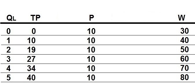
Use the data above to calculate (1) the
quantity of labor this firm will hire to maximize its profits, and
(2) the allocatively efficient quantity of labor to
hire.
Assume the firm hires labor, its only
variable resource, under monopsonistic conditions and sells its
product under competitive conditions.
Minimum Wage - Traditional
Model
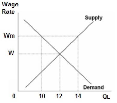
MULTIPLE CHOICE:
1. In the labor market shown above, with NO
MINIMUM WAGE, the equilibrium quantity employed will be:
A. 0 B. 10 C. 12 D. 14
2. In the labor market shown above, if the
minimum wage is set at Wm, the equilibrium quantity employed will
be:
A. 0 B. 10 C. 12 D. 14
3. In the labor market shown above, the
allocatively efficient quantity to employ is:
A. 0 B. 10 C. 12 D. 14
4. In the labor market shown above, if the
minimum wage is set at Wm, the amount of unemployment created by the
minimum wage is:
A. 2 B. 4 C. 12 D. 14
5. In the labor market shown above, if the
minimum wage is set at Wm, it will cause:
A. Employment to increase from 10 to 12
B. Employment to increase from 12 to 14
C. Employment to decrease from 14 to 12
D. Employment to decrease from 12 to 10
Minimum Wage in a Monopsony
Model
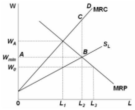
MULTIPLE CHOICE:
1. Use the figure above to answer this
question., If the minimum wage is set at Wmin, what will happen to
employment in this monopsonistic labor market?
A. Employment will decrease
B. Employment will increase
C. Employment will stay the same
D. Employment may increase but usually it tends to stay the same
2. Use the figure above to answer this
question. Senator Approximire opposes a proposal that the monopsonist
pay a minimum wage of at least Wmin stating "Even if the labor market
is monopsonistic, economic theory unambiguously demonstrates that
imposing a minimum wage causes employment to fall." Senator
Approxmire is:
A. Correct because the law of demand states that as the wage
rises, the firm demands less labor
B. Incorrect because the monopsonist would offer a wage of
WA,
which is higher than Wmin, and maintain its employment level at
L1
C. Incorrect because the monopsonist's effective MRC curve becomes
ABCD, which means that it will choose to hire more workers, from L1
to L2.
D. Correct because the graph indicates that at the wage of Wmin, the
monopsonist would not make a profit from hiring labor and so would
not hire any at all
3. Use the figure above to answer this
question,. If the minimum wage is set at Wmin then:
A. this labor market will become less efficient
B. this labor market will become more efficient
4. Use the figure above to answer this
question. The allocatively efficient quantity of labor is:
A. L1 B. L2 C. L3
Minimum Wage and Price Elasticity of Demand
for Labor Model
(Jobs are lost, but do the poor gain more
income?)
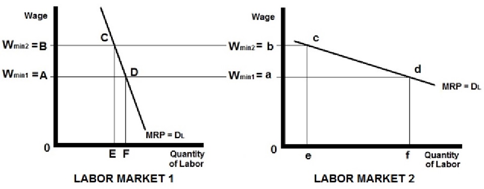
MULTIPLE CHOICE:
1. Use the figure above to answer this
question. If the minimum wage is increases from Wmin1 to Wmin2 what
will happen to the income received by minimum wage workers in Labor
Market 1?
A.decrease from 0BCD to 0ADF
B.decrease from 0ADF to 0BCD
C.increase from 0ADF to 0BCE
D.increase from 0BCE to 0ADF
2. Use the figure above to answer this
question. If the minimum wage is increases from Wmin1 to Wmin2 what
will happen to the income received by minimum wage workers?
A. Total incomes decrease for minimum wage workers in Labor
Market 1 because the demand for labor is elastic
B. Total incomes increase for minimum wage workers in Labor Market 2
because the demand for labor is elastic
C. Total incomes increase for minimum wage workers in Labor Market 1
because the demand for labor is inelastic
D. Total incomes decrease for minimum wage workers in Labor Market 2
because the demand for labor is inelastic
3. Use the figure above to answer this
question. In which labor market is the demand for labor less price
(wage) elastic?
A. Labor Market 1
B. Labor Market 2
4. Use the figure above to answer this
question. Which of the following is correct if the minimum wage is
increased from Wmin1 to Wmin2 ?
A. Total revenues increase in Labor Market 1 and decrease in
Labor Market 2
B. Total revenues decrease in Labor Market 1 and increase in Labor
Market 2
C. Total revenues increase in both labor markets
D. Total revenues decrease in both labor markets
5. So, even if raising the minimum wage
causes more unemployment, does such an increase help minimum wage
workers?
A.Yes
B. No
C. It depends on the price elasticity of demand for low skilled labor
Competitive Labor Market in a Competitve
Product Market
Competitive Labor Market in an
Imperfectly Competitive Product Market
Monopsony
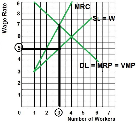
Union: Increase Demand
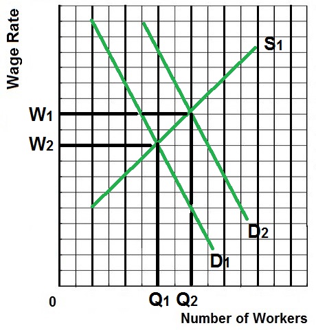
Union: Craft
(Exclusive)
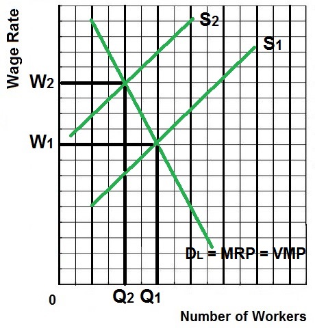
Union: Inclusive
(Industrial)
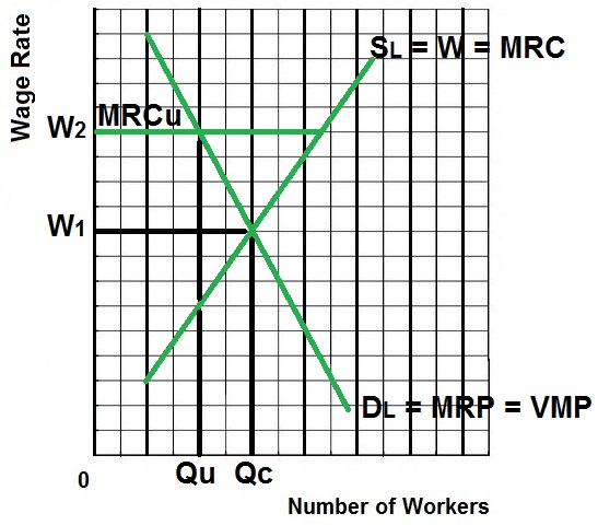
Union: Bilateral
Monopoly
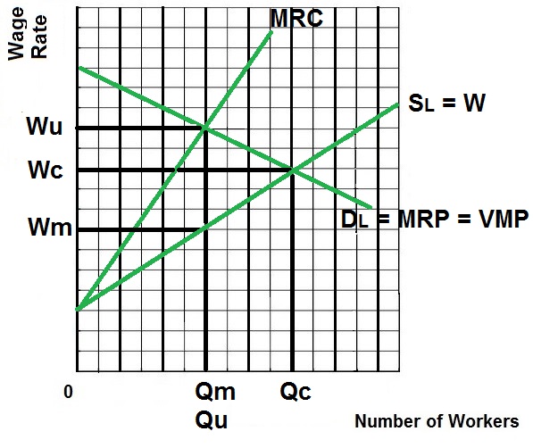
Minimum Wage Traditional Model:
employment decreases
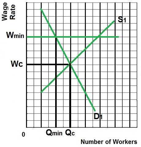
Minimum Wage in a Monopsony:
employment increases
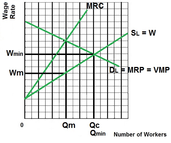
Does the Minimum Wage help the
poor?
YES if the demand for labor is inelastic
because total income increases from 0ADF to 0BCE (red to
blue)
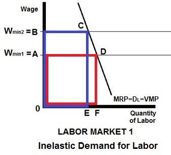
Does the Minimum Wage help the
poor?
NO if demand for labor is elastic because total
income decreases from 0adf to 0bce (red
to blue)
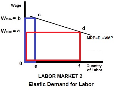
- Micro
Unit 5, Question 12: Monopsony
[2:59 YouTube ACDC Leadership]
- Micro
5.1 Market and Minimum Wage: Econ Concepts in 60 Seconds:- Economics
Lesson
[3:26 YouTube ACDC Leadership]
- Minimum
Wage Misconceptions with Jacob Clifford
[5:09 YouTube ACDC Leadership]
NOTE: These are REVIEW videos only. In order to
learn the material you must read the assigned textbook readings,
watch the assigned lecture videos, and do problems. See the
MICWEBAPP
or the LESSONS
link for these assignments.
Unit 4: Labor and Efficiency: Resource
Markets, Inequality, and Immigration
Lesson 20a: Income Inequality and
Discrimination
The gap between the rich and the poor is
getting wider and income inequality has become an important political
issue. We will learn that the 42 richest people on Earth now have the
same amount of wealth as the bottom half of the global population. 42
people have the same amount of wealth as the poorest 3.5 billion
(3,500,000,000) !
We will first look at some data on the
distribution of income and learn how to measure it.
Then we will learn two models concerning income
distribution:
1. The Case for Equality Model:
Maximizing Total Utility. This is the President Trump Example from
lesson 1b and
2. The Occupational Discrimination (Crowding) Model
The YELLOW PAGES, the LESSONS webpage, and the
MICWEBAPP have one page summaries of each of these models. You should
find them and study them.
20a Something Interesting - Why are
we studying this?
|
Jan. 2018: According to an Oxfam report just 42
people now hold as much wealth as the poorest 3.7 billion. In the
U.S., the country’s 3 richest people have the same wealth as the
poorest half of the American population.
https://www.huffingtonpost.com/entry/billionaires-oxfam-inequality_us_5a657e61e4b0022830041a7a
https://www.oxfamamerica.org/static/media/files/bp-reward-work-not-wealth-220118-en.pdf
In Jan. 2014 the number was 85 of the world's
richest people owned the same amount of wealth as the bottom half of
the global population and in Jan. 2017 it was 61 people.
Think about it. The wealth of the 42 richest
people = the wealth of the 3.5 billion poorest.
And, the gap between the rich and the poor is
widening.
20a Assignments: Readings
|
pp. 324-326, (19th, 260-262), "Marginal
Productivity Theory of Income Distribution"
pp. 465-475, (19th, 410-419), "Facts about
Income Inequality", "Causes of Income Inequality", "Income Inequality
over Time", "Equality versus Efficiency"
pp. 482-485, (19th, 426-427), "Occupational
Segregation: The Crowding Model"
Model
Summaries
Oxfam
report highlights widening income gap between rich,
poor
Researchers
Examine Gap between Rich and Poor (NPR
Morning edition, 1/28/2014) Read or listen 5:43
Guaranteed Basic Income / Universal Basic
Income
Lecture
Outline
20a Assignments: Video
Lectures
|
10.3.4 Hot
Topic: Income Distribution in the U.S.
5:20 [MyNotes]
Wealth
Inequality in America (Politizane
YouTube) 6:24
20a Outcomes - What you should
learn
|
TOPICS
- Describing Income Distribution
- Government Redistribution
- Growing Inequality
- The Equality Model (Pres. Trump Example -
lesson1d)
- The Occupational Crowding Model
- Guaranteed Basic Income
OUTCOMES
- Describe the distribution of income in the
United States (by quintile).
- Explain how Lorenz curves and Gini ratios
are used to describe income inequality.
- Discuss the impact of income mobility on
income distribution data.
- Explain the broadened concept of income,
which includes the effects of taxes and transfer payments, and how
this affects the extent of inequality of income and poverty in the
U.S.
- List causes of an unequal income
distribution.
- Describe changes and causes for the changes
in inequality since 1970.
- The "Case for Equality Model" - Understand
the connection between the Pres. Trump example of equity and the
lesson 20a "Case for Equality Model" and what is the problem with
this reasoning (the equality vs. efficiency argument)
- Occupational Discrimination - "The Crowding
Model"
- Guaranteed basic income (also called
"universal basic income" and "unconditional basic
income")
Key
Terms Flash Cards - Click Here
Key Terms:
income inequality, quintile, Lorenz
curve, Gini ratio (Gini coefficient), income mobility, transfer
payment, progressive income tax, noncash transfers,
equality-efficiency trade-off, discrimination, occupational
segregation, "President Trump example", guaranteed basic income
(also called "universal basic income" and "unconditional basic
income")
The
Case for Equality Model Click Here
The
Occupational Discrimination Model - Click Here
The Case for Equality Model of
Income Distribution
(The 5Es - President Example)
(The Utility Maximizing Distribution of Income)
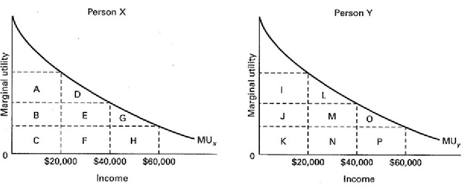
MULTIPLE CHOICE: Refer to the above diagrams
which show identical marginal utility curves for Person X and Person
Y. Assume a given income of $80,000 is initially distributed so that
Person X receives $60,000 and Person Y $20,000.
1. The marginal utility:
1. of the last dollar will be greater for
Person Y than for Person X
2. derived from the last dollar will not be comparable between the
two income receivers
3. of the last dollar will be the same for both Person X and Person
Y
4. of the last dollar will be greater for Person X than for Person
Y
2. Which is true about redistributing the
income?
1. no judgement can be made as to the effect of
a redistribution on total utility
2. this initial distribution of income is maximizing the combined
total utility of the two consumers
3. the combined total utility of the two consumers can be increased
by redistributing income from Person Y to Person X
4. the combined total utility of the two consumers can be increased
by redistributing income from Person X to Person Y
3. If this income is redistributed equally
then the total combined utility will:
1. increase by DEFGH minus LMNOP
2. increase by LMNOP minus DEFGH
3. increase by LMN minus GH
4. increase by GH minus LMN
5. decrease by GH
Occupational Discrimination
Model
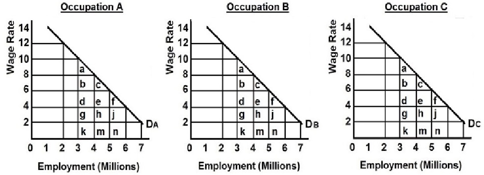
ASSUMPTIONS:
(1) the labor force is comprised of
6 million men and 6 million women workers;
(2) the economy has 3 occupations, A, B,
and C, each having identical demand curves for labor;
(3) men and women workers are homogeneous
with respect to their labor-market capabilities;
(4) women are discriminated against by
being excluded from occupations A and B and are confined to C; and
(5) aside from discrimination, the
product and labor markets are competitive, therefore D = MRP = VMP
= P x MP
QUESTION: Refer to the above diagram and
list of assumptions. If discrimination is ended what happens to
output?
Gini Ratio
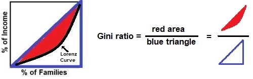
Lorenz Curve
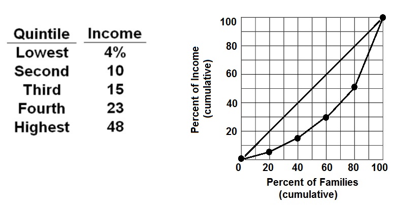
The Case for Equality = the President
Trump Example
The Utility Maximizing Distribution of Income
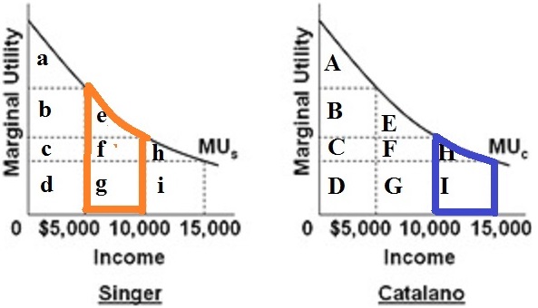
The Occupational Segregation Model of
Discrimination
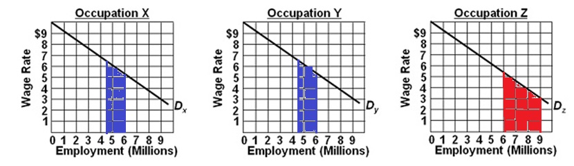
The
Case for Equality Model: Maximizing Total
Utility. (This is the President Trump
Example from lesson
1b)
The
Occupational Discrimination (Crowding) Model
- Income
and Wealth Inequality: Crash Course Economics
[10:15 YouTube CrashCourse]
NOTE: These are REVIEW videos only. In order to
learn the material you must read the assigned textbook readings,
watch the assigned lecture videos, and do problems. See the
MICWEBAPP
or the LESSONS
link for these assignments.
Unit 4: Labor and Efficiency: Resource
Markets, Inequality, and Immigration
Lesson 22a:
Immigration
Immigration is another labor issue that has
become an important political topic. We will first study some
historical data on U.S. immigration, then we will look at two
immigration models:
1. a simple immigration model showing
the "Impact on Wage Rates, Efficiency, and Output", and
2. a model showing the impact of illegal
workers in a low wage labor market
The YELLOW PAGES, the LESSONS webpage, amd the
MICWEBAPP have one page summaries of each of these models. You should
find them and study them.
22a Something Interesting - Why are
we studying this?
|
Read this short news article from 2013:
http://www.nytimes.com/2013/02/17/magazine/do-illegal-immigrants-actually-hurt-the-us-economy.html
From the eighth paragraph of the above website:
Nearly all economists, of all
political persuasions, agree that immigrants — those here
legally or not — benefit the overall economy. “That is
not controversial,” Heidi Shierholz, an economist at the
Economic Policy Institute, told me. Shierholz also said that
“there is a consensus that, on average, the incomes of
families in this country are increased by a small, but clearly
positive amount, because of immigration."
After studying this lesson you should be able
to discuss the effects of immigration on substitute resources and
complementary resources.
22a Assignments: Readings
|
pp. 513-529, (19th, Ch.
22, ALL)
Model
Summaries
"Three
Ways To Totally Transform U.S. Immigration
Policy" NPR, Planet Money, Feb. 21,
2013
1. The Best And The Brightest
2. The Highest Bidder
3. Let 'Em In
"Do
Illegal Immigrants Actually Hurt the U.S.
Economy?" Adam Davidson, New York
Times, Feb. 12, 2013
"Give
Me Your Tired, Your Poor, and Your Economists,
Too" By N. Gregory Mankiw, Feb. 9,
2013
Lecture
Outline
22a Assignments: Video
Lectures
|
- Costs,
Benefits and How Best to Respond -
Professor Richard D Wolff (RichardDWolff 6:59)
- Immigrants do depress wages
- Immigrants are not a net gain
- Allow immigrants but support labor unions
-
CNN
Report on the economics of immigration
(2:24)
22a Outcomes - What you should
learn
|
TOPICS
- Economic immigration
- Economic effects of immigration
- The illegal immigration debate
OUTCOMES
- Understand the historical pattern of legal
and illegal immigration the United States.
- List the factors influencing the decision
to migrate.
- Understand the potential impact immigration
can have on wage rates, efficiency, and output. "Impact on Wage
Rates, Efficiency, and Output"
- Understand how immigration can affect
income shares.
- Identify potential complications with the
traditional model of immigration: Remittances, Full-Employment or
Unemployment, and Complements and Substitutes.
- Understand the effect immigration to the
United States has on Federal, State, and Local governments' fiscal
position.
- Understand the illegal immigration debate
in the context of " job crowding-out". ["Impact of Illegal
Workers in a Low Wage Labor Market"]
- Explain the potential price effects that
illegal immigration can have on an economy.
- Understand the concept of 'optimal'
immigration
- Do Illegal Immigrants Actually Hurt the
U.S. Economy?
http://www.nytimes.com/2013/02/17/magazine/do-illegal-immigrants-actually-hurt-the-us-economy.html
- Discuss the effect on substitute
resources and complementary resources on employment
From paragraph 8 of the above website:
"Nearly all economists, of all political persuasions, agree
that immigrants — those here legally or not — benefit
the overall economy. “That is not controversial,”
Heidi Shierholz, an economist at the Economic Policy Institute,
told me. Shierholz also said that “there is a consensus
that, on average, the incomes of families in this country are
increased by a small, but clearly positive amount, because of
immigration.”
Comments?
Key
Terms Flash Cards - Click Here
Key Terms:
economic immigrants, legal immigrants,
illegal immigrants, human capital, beaten paths, backflows,
efficiency gains from migration, brain drain, remittances,
complementary resources, substitute resources, fiscal
impacts
Simple
Immigration Model - Click Here
Illegal
Immigration Model - Click Here
Economic Effects of Immigration - The
Simple Immigration Model
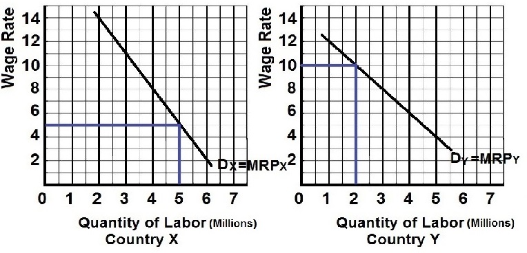
See the assumptions below, then answer these
questions:
1. How many will migrate from the low
wage country X to the high wage country Y?
2. What happens to the wage rate in X and in Y?
3. What happens to output in X, in Y, and total output?
4. What would happen to output if initially there was unemployment
in low wage country X?
5. How do remittances affect low wage country X?
Assumptions:
1. Dx is the demand for labor in
country X. Dy is the demand for labor in country Y.
2. Before migration the labor force in country X is 5 and the
labor force in country Y is 2.
3. Neither country has any unemployment.
4. Migration (1) has no costs, (2) occurs only in response to wage
differentials, and (3) is unimpeded by law in both countries.
5. Labor markets and product markets are competitive so Dlabor =
MRP = VMP = P x MP
Answer:
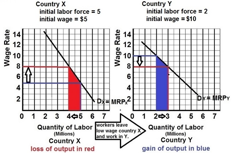
Impact of Illegal workers in a Low Wage
Market - The Illegal Immigration Model
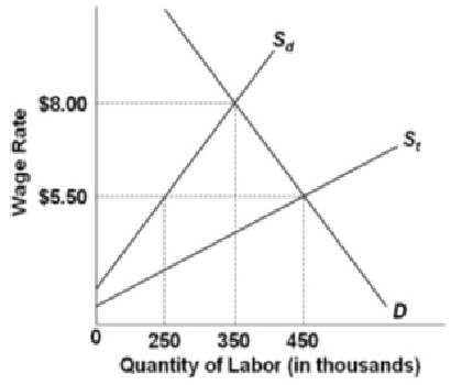
MULTIPLE CHOICE:
Assumptions:
1) Employers in this market are
willing and able to ignore minimum wage laws;
2) Sd represents the supply of domestically-born and legal
immigrant workers;
3) St represents the total supply of workers in this labor market
(St = Sd + illegal immigrants);
4) Unless otherwise stated, illegal immigration is not effectively
blocked by the government.
1. Refer to the above figure. The
equilibrium wage and level of employment are, respectively:
1. $5.50 and 250,000
2. $5.50 and 350,000
3. $8.00 and 350,000
4. $5.50 and 450,000
2. Refer to the above figure. How many
domestically-born and legal immigrant workers will be hired at
equilibrium?
1. 200,000
2. 250,000
3. 350,000
4. 450,000
3. Refer to the above figure. How many
illegal immigrant workers will be hired at equilibrium?
1. 200,000
2. 250,000
3. 350,000
4. 450,000
4. Refer to the above figure. If the
government effectively prevents illegal immigrants from working in
this labor market, the equilibrium wage and level of employment are,
respectively:
1. $5.50 and 250,000
2. $5.50 and 350,000
3. $8 and 350,000
4. $5.50 and 450,000
5. Refer to the above figure. Assume
initially that government does not effectively block illegal
immigration. If the government then finds a way to prevent all
illegal immigrants from working in this labor market:
1. 100,000 domestically-born workers
will gain employment at the expense of 200,000 illegal
immigrants.
2. 200,000 domestically-born workers will gain employment at the
expense of 200,000 illegal immigrants.
3. 100,000 domestically-born workers will gain employment at the
expense of 250,000 illegal immigrants.
4. 100,000 domestically-born workers will gain employment at the
expense of 100,000 illegal immigrants.
Simple Immigration
Model
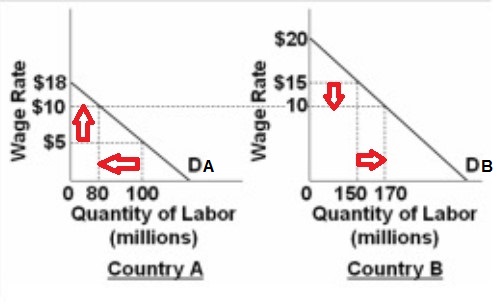
Impact of Illegal Workers in a Low Wage
Labor Market
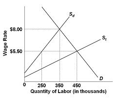
A
simple immigration model showing the "Impact on Wage Rates,
Efficiency, and Output"
A
model showing the impact of illegal workers in a low wage labor
market
The
Economics of Immigration: Crash Course Econ #33
[11:20 YouTube CrashCourse Economics]
NOTE: These are REVIEW videos only. In order to
learn the material you must read the assigned textbook readings,
watch the assigned lecture videos, and do problems. See the
MICWEBAPP
or the LESSONS
link for these assignments.