OUTLINE -- CHAPTERS 6 & 12
A Model of the Macro Economy: Aggregate Demand and Supply
Lectures
12a Introduction to Macroeconomics and Aggregate Demand
(AD)
|
I. Structural Adjustment Policies
1. Privatization
2. Promotion of Competition
3. Limited and Reoriented Role for Government
4. Price Reform: Removing Controls
5. Joining the World Economy
6. Macroeconomic
Stability
II. Introduction
A. Macroeconomics vs. Microeconomics
1. definition -- economics
2. definition -- macroeconomics
3. definition -- microeconomics
B. Macroeconomics Issues
1. full employment (or UE)
2. price stability (or IN)
3. economic growth (EG)
C. Chapter 6: Macroeconomic Concepts and the role of Price
"Stickiness"
1. How well is the economy doing? - Performance and
Policy
a. Real GDP (real Gross Domestic Output)
(1) nominal GDP
- total dollar value of all final goods
and services produced within the borders of a country
using their current prices during the year that
they were produced
- PROBLEM: nominal GDP can increase from year to
year even if there is no increase in output
(2) real GDP
- measures the total dollar value of a
final goods and services produced within the borders
of a country in a year
- measures the quantity being produced
- USEFUL to see if a country's output is
growing
- real GDP uses THIS YEAR's QUANTITY and BASE
YEAR PRICES (prices do not change)
(3) GDP = C + I + G + Xn
b. Unemployment
FULL employment:
- 5 Es Definition: full employment is
using all available resources
- Common Definition: all available labor is
employed
UNemployment (UE)
- occurs when a person is not working,
but looking
- "UE is a waste"
c. Inflation
an increase in the overall level of
prices
2. The Miracle of Modern Economic Growth
a. growth before the industrial revolution
(1) output growth increased slowly AND
populations increased slowly
(2) output per capita growth stayed about the same
= NO GROWTH for hundreds of years or more
(3) result:
(a) no change in living standards in a
given place
(b) little difference between living standards
between places
b. modern economic growth - "Rapid economic growth is
a modern phenomenon")
(1) industrial revolution: output grows
faster than population
(a) beginning around 1750 in England
(b) not all countries
(c) even small increases in output result in
large increases in living standards over time
- rule of 70
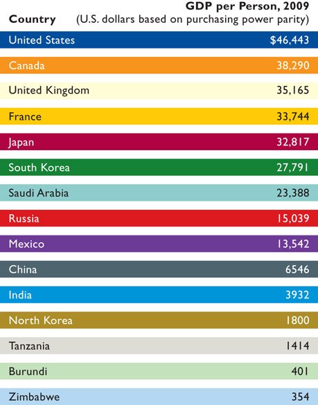
- If a $10,000 GDP per capita increases by 2%
a year
- how long will it take to double to
$20,000?
- how long will it take to quadruple to
$40,000?
- how long will it take to reach
$80,000?
(d) RESULTS:
- higher living standards in places
- vast differences in living standards
- GDP per capita or per person is a measure
of the standard of living of a country
- GDP per capita = GDP / population
3. Savings, Investment, and Choosing between Present and
Future Consumption
a. Review: Production Possibilities Model:
Present Choices Future Possibilities
b. Saving occurs when current consumption is
less than current output
(or when current spending is less than current
income)
c. Investment
- happens when resources are devoted to increasing
future output
- the only way for there to be investment is for
there to be saving
- WARNING: "investment" in economics has a different
definition
(1) financial investment
- the purchase of financial assets (stocks,
bonds, mutual funds) or a real assets (houses, land
factories) or the building of such assets in the
expectation of financial gain
(2) economic investment
- spending for the production and accumulation of
capital (capital resources)
d. economic investment is ultimately limited by the
amount of savings, and more savings now depends on less
consumption now
e. the role of banks
- households are the principle savers
- but businesses are the main investors
- Banks are then the "financial
intermediaries"
4. Uncertainty, Expectations, Demand Shocks, and Supply
Shocks
a. definitions
- demand shocks: unexpected changes in the demand
for goods and services
- supply shocks: unexpected changes in the supply of
goods and services
- "shock" means "unexpected"
- shocks can be positive or negative
b. "Economists believe that most short-run
fluctuations in GDP are the result of demand shocks"
[NOTE: there are also supply shocks, but we will
concentrate more on demand shocks]
(1) demand shocks and flexible prices:
producing the full employment output
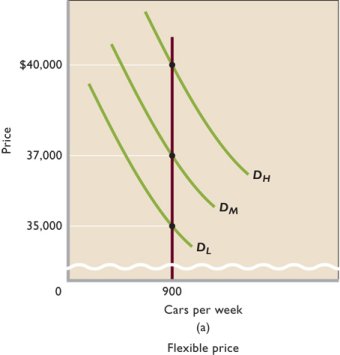
For the economy: if the prices of goods
and services could always adjust quickly to
unexpected changes in demand, then the economy
could always produce at its optimal capacity since
prices would adjust to ensure that the quantity
demanded for each good would always equal the
quantity supplied.
(2) demand shocks and sticky prices: fluctuations
in GDP and employment
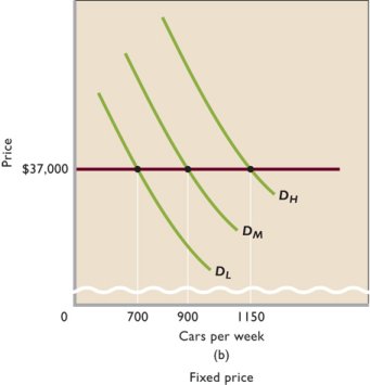
For businesses: if prices are inflexible
then they respond to demand shocks by adjusting output
or maintaining and inventory, but if the shock
continues, output, and employment, will have to
change
For the economy: if prices are inflexible than
the economy adjusts to demand shocks by changing
output and hence production and employment
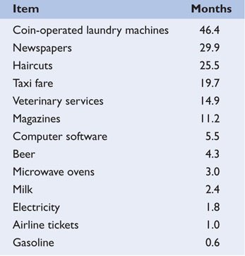
5. How Sticky are Prices?
- if "sticky prices' explain fluctuations in output and
employment in the short run, how sticky are prices?
- it varies (see table below)
- WHY?
- consumers like it
- businesses fear a price war
6. Macroeconomic models and Price Stickiness
- price stickiness changes over time
- "stuck prices" only in the extreme short
run
- "sticky prices" in the short run
- "flexible prices" in the longer run
- different macro models for different lengths of time
because the economy behaves differently over different
lengths of time
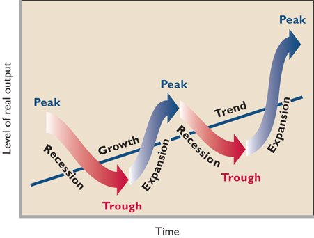
D. The Business Cycle
1. phases of the cycle
a. peak
b. recession
c. trough
d. expansion (often called "recovery")
2. the business cycle and the macro economic issues
3. causes of the business cycle: changes in aggregate
expenditures (demand shocks)
4. secular trend
5. For a table of the US Business cycles: http://www.nber.org/cycles.html
E. Chapter 12: A Model of the Macro Economy: AD and
AS
1. Chapter 3: D and S
2. Chapter 12: AD and AS
III. Aggregate Demand
A. Definition
B. Real Domestic Output and the Price Level
C. Graphically: downsloping -- why?
1. wealth effect
2. interest-rate effect
3. foreign purchases effect
3. increase and decrease in AD
|
AD INCREASE
|
AD DECREASE
|
3. So what causes changes in AD?
a. determinants of AD: FROM
CLASS
- change in consumer spending (C)
- change in Investment spending (I)
- change in Government spending (G)
- change in Net Exports (Xn)
- change in Money Supply (S)
- change in Taxes (T)
- change in Saving (S)
b. determinants of AD: FROM TEXT
1) C = consumer spending (and saving)
1) consumer wealth
2) consumer expectations
3) taxes
4) consumer indebtedness
I like the determinant "consumer debt"
better than the "household borrowing" determinant
mentioned in the textbook. The authors of our
textbook say:
Household borrowing 
 C
AD
C
AD
Household borrowing  C
AD
C
AD
I think what they are really saying is:
Interest rates
Household borrowing
C
AD
Interest rates
Household borrowing
C
AD
But they also say, "The aggregate demand curve
will also shift to the left (
AD)
if consumers increase their savings rates in order
to pay off their debts".
So why then do I prefer "consumer debt" as a
determinant of AD? Because newspapers discuss
it.
http://www.nytimes.com/2009/08/08/business/08credit.html
If consumers are greatly in debt they may be
expected to begin to pay off those debts which
will: S
C
AD
If consumer debt is going down, as it was during
2009, we might expect that in the near future: S
C
AD
2) I = investment spending
1) interest rates (money supply)
I know the textbook does not mention
"money supply", but it will in unit 3. So, we might
as well learn it now.
2) profit expectations on investment
projects
3) business taxes
4) technology
5) degree of excess capacity
3) G = government spending
4) Xn = net export spending
1) net income abroad
2) exchange rates
12b Aggregate Supply and Macroeconomic Equilibrium
|
IV. Aggregate Supply (AS)
A. Definition [lecture]
B. Graphically
1. AS in the Immediate Short Run
a. assumption: both input prices and output
prices are fixed
b. can be a few days to a few months depending on the type
of firm
c. input prices are often fixed by contract; e.g. wage and
salary contracts
d. output prices are often fixed when firms set their "list"
price and follow it for awhile, also : catalog prices
e. graph
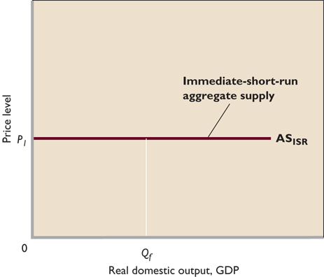
f. Result: the total output supplied depend on total
spending (AD) until the firm is able to change its
prices
2. AS in the Short Run
a. input prices are fixed (or highly
inflexible), but output prices can vary
b. not really a certain time period, the length of the short
run depends on whether input prices (like wage contracts)
can change
c. graph
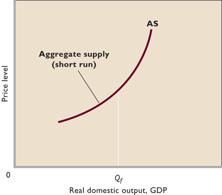
d. shape:
1. initially the price level rises slowly as
output increases because since the economy is operating
fall below its capacity (Qf) there are large amounts of
unused resources available that firms can use without
causing its cost per unit to increase
2. as we get near to, or beyond, the full
employment level of output the price level rises more
quickly because costs per unit rise more quickly
(a) example adding more workers to a fixed
size factory (it will get crowded) - result: higher
per unit costs
(b) or adding onto the factory, but few
additional workers are available to work there -
result: higher per unit costs
3. AS in the Long Run
a. both input (including wages) and output
prices are fully flexible
b. graph
c. shape:
(1) vertical meaning that in the long run the
economy will be producing the full employment level of
output no matter what the price level is -- why?
(2) if aggregate spending (demand) is high firms
want to produce more than the full employment level
because of higher profits, BUT this will cause workers to
demand higher wages causing profits to drop and firms
will then no longer have the incentive to produce
more
C. A Compound AS Graph
1. upsloping
2. shape
a. Keynesian (horizontal) range
b. classical (vertical) range
c. intermediate (upsloping) range
3. aggregate supply and full employment
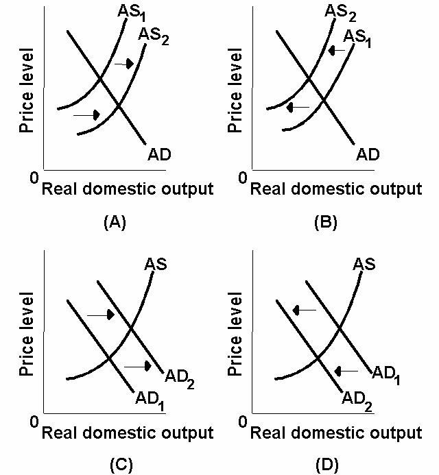
2. increase and decrease in AS
AS INCREASE
AS DECREASE
5. So what causes changes
in AS?
a. determinants of AS
1) change in input prices
a) labor
b) land (OPEC)
http://news.bbc.co.uk/hi/english/business/the_economy/newsid_300000/300492.stm
c) capital
d) entrepreneurial ability
2) changes in the productivity of resource
a) productivity
b) production
c) productive efficiency
3) legal-institutional environment
a) business taxes and subsidies
b) government regulation (red-tape)
V. Macroeconomic Equilibrium
A. Equilibrium
1. equilibrium price level
2. equilibrium real domestic output
B. Changes in AD and the Macroeconomic Issues
1. Increase in AD
a. UE decreases
a. IN increases = demand-pull inflation
2. Decrease in AD
a. UE increases
b. inflation decreases
c. ratchet effect: the price-level may not decrease
(but IN does decrease)
1) graphically
2) causes of the ratchet effect
a) fear of price wars
b) menu costs
c) wage contracts
e) morale and productivity, training investments
f) minimum wage
3. REVIEW (12a) So what causes changes in AD?
a. determinants of AD: FROM
CLASS
- change in consumer spending (C)
- change in Investment spending (I)
- change in Government spending (G)
- change in Net Exports (Xn)
- change in Money Supply (S)
- change in Taxes (T)
- change in Saving (S)
b. determinants of AD: FROM TEXT
1) C = consumer spending (and saving)
1) consumer wealth
2) consumer expectations
3) taxes
4) consumer indebtedness
I like the determinant "consumer debt"
better than the "household borrowing" determinant
mentioned in the textbook. The authors of our
textbook say:
Household borrowing
C
AD
Household borrowing
C
AD
I think what they are really saying is:
Interest rates
Household borrowing
C
AD
Interest rates
Household borrowing
C
AD
But they also say, "The aggregate demand curve
will also shift to the left (
AD)
if consumers increase their savings rates in order
to pay off their debts".
So why then do I prefer "consumer debt" as a
determinant of AD? Because newspapers discuss
it.
http://www.nytimes.com/2009/08/08/business/08credit.html
If consumers are greatly in debt they may be
expected to begin to pay off those debts which
will: S
C
AD
If consumer debt is going down, as it was during
2009, we might expect that in the near future: S
C
AD
2) I = investment spending
1) interest rates (money supply)
I know the textbook does not mention
"money supply", but it will in unit 3. So, we might
as well learn it now.
2) profit expectations on investment
projects
3) business taxes
4) technology
5) degree of excess capacity
3) G = government spending
4) Xn = net export spending
1) net income abroad
2) exchange rates
C. Changes in AS and the Macroeconomic Issues
1. Increase in AS
a) UE decreases
b) IN decreases
2. decrease in AS
a) IN increases -- called cost-push inflation
b) UE increases
c) "stagflation" = increase in UE and increase in
IN
3. REVIEW (12a): So what causes changes
in AS?
a. determinants of AS
1) change in input prices
a) labor
b) land (OPEC)
http://news.bbc.co.uk/hi/english/business/the_economy/newsid_300000/300492.stm
c) capital
d) entrepreneurial ability
2) changes in the productivity of resource
a) productivity
b) production
c) productive efficiency
3) legal-institutional environment
a) business taxes and subsidies
b) government regulation (red-tape)
D. What about economic growth (EG) ?
1. Review: What do we already know about Economic
Growth?
a. Definition from chapter 1:
- 5Es Definition
- Increasing our ABILITY to Produce or Increasing
POTENTIAL output
- one of the 5Es of economics to maximize
satisfaction or reducing SCARCITY
- causes
- more resources
- better resources
- better technology
- Production Possibilities Graph
2. Two (or Three) Definitions
- Increasing the ABILITY to produce = increasing
our potential
- Increasing Real GDP = producing more =
achieving our potential
- Increasing GDP per capita = increasing output
PER PERSON
a. Increasing our ABILITY to Produce
- INCREASING THE POTENTIAL
- Ch. 1 Definition
- "economic growth" on the 5Es chart
- shifts production possibilities curve outward
- AD and AS model increases AS
- Causes of this type of EG (increase
Potential):
- change in input prices (more
resources)
- changes in the productivity of resource (better
resources, better technology)
- legal-institutional environment
b. Increasing Real GDP
- increasing output = definition often used in the news
= producing more
- "Ch. 8 definition"
- ACHIEVING OUR POTENTIAL
- achieving "full employment" and "productive
efficiency"
- production possibilities curve:
- AD and AS model: AD
c. A third definition of EG: increasing GDP per capita;
we will discuss in ch. 9
VI. USING AS/AD
A. Yellow Pages
b. Articles used in class:
12c Stabilization Policies and AS/AD in the Long Run
|
VII. Macroeconomic Policies
A. Economic Functions of Government: Five Reasons for
Government Involvement (lesson 2b)
1. legal and social framework
2. maintaining competition
3. redistribution of income (correcting market
failure to achieve equity)
4. reallocation of resources (correcting market
failure to achieve efficiency)
5. stabilizing unemployment
and inflation and promoting economic growth
B. Stabilization Policies ("Promoting Stability" )
1. definition:
- a structural adjustment policy
- Def. - a gov't policy designed to lower unemployment
and/or inflation. to "stabilize the business cycle
2. Stabilization is one of the roles of government in
market economy
C. Demand-Management
1. definition: policies where the government
changes AD in order to reduce UE or IN
2. tools: AD curve shifters controlled by the
government
- change government purchases (G)
- change taxes (T)
- change interest rates by changing the money supply
(MS)
3. two types of demand management policies: fiscal policy
(FP) and monetary policy (MP)
a. fiscal policy (FP)
- where the gov't use changes in G and/or T
- conducted by the congress and the
president
- there are 2 types of FP
1) expansionary FP
- FP that fights UE
- tools: increase G or decrease T
- result: increase AD and thereby decrease
UE
- but: may result in some IN
2) contractionary FP
- FP that fights IN
- tools: increase T or decrease G
- result: decrease AD and thereby decrease
IN
- but: may result in some UE
b. monetary policy (MP) (Ch. 16)
1) easy money policy
- occurs when the Fed tries to increase money
supply in order to stimulate the economy.
- also called expansionary MP
- goal is to reduce UE
- may cause some IN
- HOW:
- increase money supply causes
- lower interest rates which causes
- more investment which causes
- increase in AD
- Graph:
2) tight money policy
- occurs when the Fed tries to decrease money
supply in order to slow down the economy.
- also called contractionary MP
- goal is to reduce IN
- may cause some UE
- HOW:
- decrease money supply causes
- higher interest rates which causes
- less investment which causes
- decrease in AD
- Graph:
3. AD policies and the AS curve
the effectiveness of demand management policy
depends on where the economy is on the AS curve
D. "Supply-Side Economics" ( "Taxation and Aggregate Supply"
)
1. Increase AS to decrease UE AND to
decrease IN
2. Graph
2. AS curve shifters (review):
a. change in input prices
b. changes in the productivity of resource
c. legal-institutional environment: business taxes
and government regulation (red-tape)
Problem: the government has little control over
AS
3. Four Supply Side Government Policies
a. lower marginal INCOME tax rates increase the
incentives to work
- Lower marginal tax rates may encourage more people to
enter the labor force.
- Lower marginal tax rates may encourage more people to
to work longer.
- Lower marginal tax rates may encourage more people to
postpone retirement.
- Lower marginal tax rates may encourage more people to
work harder.
- This would increase AS
- NOTE: this also increases AD.
- Many economists would argue that the effect on AD
is quicker and more direct and that the effect on AS is
slower and more uncertain
b. lower marginal tax rates on income earned from
savings
- The rewards for saving are increased by lower
marginal tax rates, and more saving means more investment
in new technology and higher productivity
- This would increase AS
c. lower tax rates on income earned from capital
(capital gains)
- The rewards investing in new technologies are
increased and productivity increases
- This would increase AS
d. government deregulation
4. Supply-side Economics and the Budget Deficit
a. Question: Does a decrease in tax rates
increase or decrease the government budget
deficit?
b. Supply-Side supporters argue that it could decrease
the deficit by increasing government revenue
c. Supply Side Policies and the Laffer Curve
d. Criticisms of the Laffer Curve
1) the impact of tax cuts on incentives to
work may be small
- some people work more
- some people work less = buy more
leisure
2) most economists think that the demand side
effects of tax cuts are more immediate and
certain
3) it depends where you are on the laffer curve
e. Consensus:
- there seems to be a general, but not universal,
agreement among economicts theat the US tax rates are
below "m" on the laffer curve above so continued tax cuts
probably will not increase revenues
- there are some supply-side effects of changes in
tax rates that must be considered.
VIII. Long Run Aggregate Supply
[lecture]
A. Define LRAS
- Assumption: both input and output prices are flexible.
- AS graph is vertical meaning that in the long run the
economy will produce the full employment level of output no
matter what the price level is. Why?
- If people are willing to buy more by paying more you would
think that firms will want to produce more. But if in order to
produce more they must also pay more for resources (since all
are already being used and they will have to pay more to draw
them away from other firms) then input prices will rise and
there is no increase in profits to encourage firms to produce
more.
B. Graph
C. Why?
1. Short Run AS and AD achieving full
employment:
2. The LRAS curve will occur at the full employment
(potential) level of output
3. WHY?
a. If AD increases:
- price level increases (equilibrium moves from a to
b on the graph below)
- price of resources will increase
- short run AS will decrease(equilibrium moves from
b to c on the graph below)
- RESULT: higher price level but THE SAME LEVEL OF
RDO
B. If AD decreases:
- price level decreases (equilibrium moves from a to
b on the graph below)
- price of resources will decrease
- short run AS will increase (equilibrium moves from
b to c on the graph below)
- RESULT: lower price level but THE SAME LEVEL OF
RDO
VIII. Historical Review of the U.S.
Economy
A. Depression
B. W.W.II Boom
D. Vietnam War Inflation
E. Monetary Restraint: 1979-1982
F. Aggregate Supply Shocks in the 1970s & Early 1980s:
Stagflation
1. OPEC and energy prices
2. agricultural shortfalls
3. depreciated dollar
4. demise of wage-price controls
5. productivity decline
6. inflationary expectations and wages
G. Financial Crises 2007
UNEMPLOYMENT RATE in the U.S.
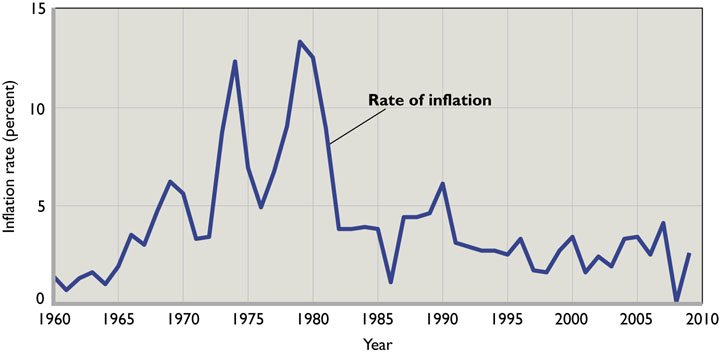
INFLATION RATE in the U.S.
X. The Phillips Curve and the Inflation - Unemployment
Tradeoff
A. Both low inflation and low unemployment are major
goals. But are they compatible?
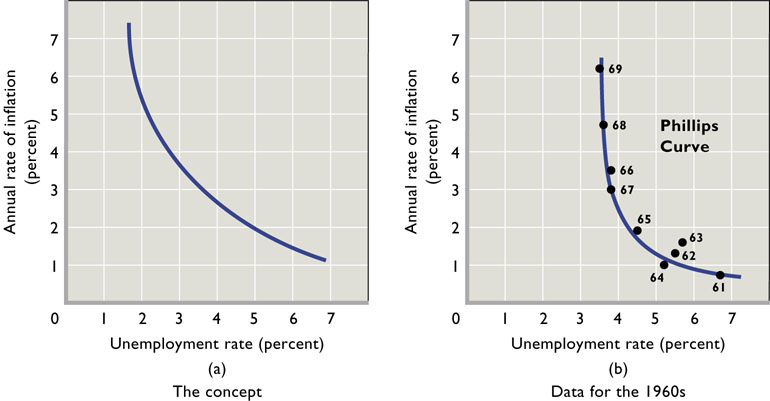
B. The Phillips Curve is named after A.W. Phillips, who
developed his theory in Great Britain by observing the British
relationship between unemployment and wage inflation. See figure
18.8:
Figure 18.8
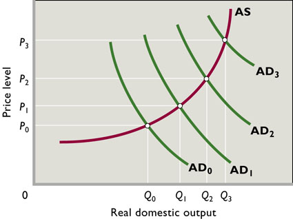
C. The basic idea is that given the short run aggregate
supply curve, an increase in aggregate demand will cause the price
level to increase and real output to expand, and the reverse for a
decrease in AD. (Figure 18.9)
Figure 18.9
D.This tradeoff between output and inflation does not occur
over long time periods.
E. Empirical work in the 1960s verified the inverse
relationship between the unemployment rate and the rate of
inflation in the United States for 1961-1969. (See Figure
18.8b)
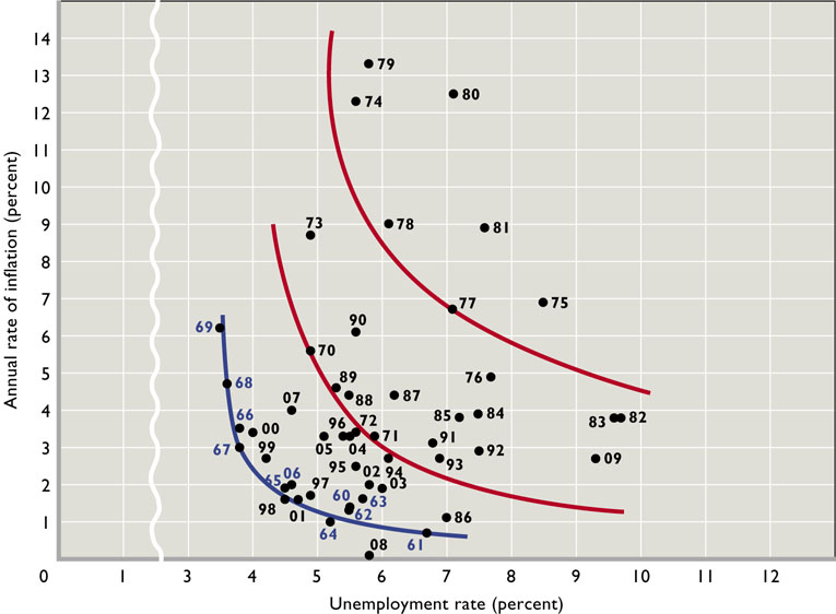
F. The stable Phillips Curve of the 1960s gave way to great
instability of the curve in the 1970s and 1980s. The obvious
inverse relationship of 1961-1969 had become obscure and highly
questionable. (See Figure 18.10)
1. In the 1970s the economy experienced increasing
inflation and rising unemployment: stagflation.
2. At best, the data in Figure 18.10 suggest a less desirable
combination of unemployment and inflation. At worse, the data
imply no predictable trade off between unemployment and
inflation.
G. Adverse aggregate supply shocks-the stagflation of the
1970s and early 1980s may have been caused by a series of adverse
aggregate supply shocks. (Rapid and significant increases in
resource costs.)
1. The most significant of these supply shocks was
a quadrupling of oil prices by the Organization of Petroleum
Exporting Countries (OPEC).
2. Other factors included agricultural shortfalls, a greatly
depreciated dollar, wage increases and declining
productivity.
3. Leftward shifts of the short run aggregate supply curve make
a difference. The Phillips Curve trade off is derived from
shifting the aggregate demand curve along a stable short- run
aggregate supply curve. (See Figure 18.8)
4. The "Great Stagflation" of the 1970s made it clear that the
Phillips Curve did not represent a stable
inflation/unemployment relationship.
H. Stagflation's Demise.
1. Another look at Figure 18.10 reveals a generally
inward movement of the inflation/unemployment points between
1982 and 1989.
2. The recession of 1981-1982, largely caused by a tight money
policy, reduced double-digit inflation and raised the
unemployment rate to 9.5% in 1982.
3. With so many workers unemployed, wage increases were smaller
and in some cases reduced wages were accepted.
4. Firms restrained their price increases to try to retain
their relative shares of diminished markets.
5. Foreign competition throughout this period held down wages
and price hikes.
6. Deregulation of the airline and trucking industries also
resulted in wage and price reductions.
7. A significant decline in OPEC's monopoly power produced a
stunning fall in the price of oil.
I. Global Perspective 35.1 portrays the "misery index" in
1999-2009 for several nations. The index adds unemployment and
inflation rates.