
|
Unit 1: ECONOMICS and
GLOBALIZATION
- 1a
- Introduction to the Course
- 1b
- What is Economics and the 5Es
- 1c
- Making Choices: Production Possibilities (PPC) and
Benefit-Cost Analysis (BCA)
- 2a
- Economic Systems and Globalization
- 2b
- Role of Government and Government Finance
- 3a
- Demand
- 3b
- Supply
- 3c
- Market Equilibrium and Efficiency
- 20a
-Why we Trade: Comparative Advantage
- 20b
- International Trade and Foreign Exchange
Markets
Unit 2: INTRO. TO
MACROECONOMICS
Unit 3: MACROECONOMIC
POLICY

Unit 1: ECONOMICS and GLOBALIZATION
|
Unit 2: INTRO. TO MACROECONOMICS |
Unit 3: MACROECONOMIC POLICY |
Unit 1: Economics and
Globalization
Lesson 1a: The Class and the
Math
Welcome to ECO 212!
1a Introduction
This course will cover the area of economics commonly defined as macroeconomics. The main goal of macroeconomics is to gain a better understanding of the causes of, and remedies for, UNEMPLOYMENT (UE) and INFLATION (IN), as well as the factors that affect ECONOMIC GROWTH (EG). We will also discuss the two types of economic growth, what I like to call "ACHIEVING THE POTENTIAL" and "INCREASING THE POTENTIAL".
Please buy the textbook as soon as possible. If you buy your textbook online, order it today. See the syllabus for the correct textbook. The textbook should cost less than $30 if you buy it online.
While you wait for your textbook to arrive there is still some work that you can do.
To begin, I suggest you do the following:
- read the syllabus
- check out our Blackboard site. Click on the menu links and see what is there
- take the Syllabus Quiz (see link on Blackboard)
- you may also begin some of the chapter 1 assignments,+ see: LESSONS
+ especially the online reading: The 5Es of Economics
Email me or use the Blackboard Discussion Board if you have questions.
Many students end up dropping or failing this course due to the lack of basic math skills. If your math skills are weak you should consider building them before taking this course. If you are required to take MTH 060 or MTH 082 and have not yet done so, do not take this economics course until you have successfully completed one of them.
I have posted a math quiz on our Blackboard site. Take the math quiz on Blackboard. If you score less then 14 or 15, consider dropping ECO 212 and taking a math class first.
Good luck and start studying.
Optional: a funny look at some major ideas of economics by
the Stand-up Economist.
1a Something Interesting - Why are we
studying this?
Principles
of economics, translated
https://www.youtube.com/watch?v=VVp8UGjECt4
*NOTE: There will be a short case study for most lessons ("Something Interesting - Why are we studying this?"). The case study does not include everything from the lesson but it will highlight an interesting and important topic. The case studies are meant to grab your attention and help you APPLY a concept from the lesson to a real world issue. At first the case study may not make sense. In fact, many will appear contrary to common sense, (like why are high prices GOOD for the people suffering from a natural disaster), but after finishing the lesson you should have a better understanding of the case study or ask for help in class or on the Blackboard discussion board.
Read: Syllabus
1a Assignments: Readings
20th: Ch. 1, pp. 4-8, (19th: pp. 3-7) "The Economic Perspective", "Theories Principles and Models", "Microeconomics and Macroeconomics",
Ch.1, Appendix on Graphing
WHAT IS ECONOMICS: THE STUDY OF SCARCITY
1a Assignments: Video
Lectures
- 1.1.1 Scarcity - Defining Economics 6:35 [MyNotes]
- 1.1.2 What Economists Do 13:20 [MyNotes]
- 1.1.3 Macroeconomics and Microeconomics 11:21 [MyNotes]
- EconMovies- Episode 1: Star Wars (Scarcity, Choices, and Exchange)
REVIEW OF GRAPHING CONCEPTS
- 1.2.1 Using Graphs to Understand Direct Relationships 9:50 [MyNotes]
- 1.2.2 Plotting A Linear Relationship Between Two Variables 9:57 [MyNotes]
- 1.2.3 Changing the Intercept of a Linear Function 8:42 [MyNotes]
- 1.2.4 Understanding the Slope of a Linear Function 7:28 [MyNotes]
OPTIONAL:
- Khan Academy Exercise: Graphing Points
- Khan Academy Exercise: Graphing Points 2
TOPICS
1a Outcomes - What you should
learn
- Introduction to the course
- What is Economics?
- Basic math and graphing
- Math Quiz
OUTCOMES
- Basic math skills
- How to find class information
- Explain and illustrate a direct relationship between two variables, and define and identify a positive sloping curve. (Appendix)
- Explain and illustrate an inverse relationship between two variables, and define and identify a negative slope. (Appendix)
- Be able to calculate the slope of a line.
- Define economics and describe the four
components of the definition:
- social science
- choice
- scarcity
- maximizing satisfaction
- What are economic models and why do economists use them?
- Explain the importance of ceteris paribus in formulating economic principles.
- Differentiate between microeconomics and macroeconomics.
- Define and give examples of the four types of resources (factors of production) and know the payment for each
Key
Terms Flash Cards - Class Activities - Click Here
1a Key Terms
Key Terms Flash Cards - What is Economics? - Click Here
Key Terms Flash Cards - Math - Click Here
Key Terms:
CLASS ACTIVITIES: Pre-quiz, Clicker Quiz, Required Activity, Yellow Pages, Tomlinson Videos on Thinkwell, Video Notes, LESSONS webpage,WHAT IS ECONOMICS?: economics, economic model, microeconomics, macroeconomics, utility, rational choice, opportunity cost, benefit-cost analysis (marginal analysis), ceteris paribus (other things equal assumption),
MATH: direct (positive) relationship, inverse (negative) relationship, slope of a line, positive slope, negative slope, origin, horizontal (x) axis, vertical (y) axis
Slope = rise/run
1a Key Formulas
Slope = vertical change / horizontal change
Slope = marginal value of the total
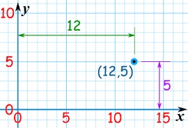
Any Point on a Graph Represents Two Numbers
1a Key Graphs
Direct Relationship
Inverse Relationship
Calculating Slope
Episode
5A: Models & Theories
1a Review Videos
[3:26 YouTube mjmfoodie]
Episode
6: Graph Review
[4:22 YouTube mjmfoodie]
NOTE: These are REVIEW videos only. In order to learn the material you must read the assigned textbook readings, watch the assigned lecture videos, and do problems. See the MACWEBAPP or the LESSONS link for these assignments.
Unit 1: Economics and
Globalization
Lesson 1b: How to Reduce Scarcity -
Introduction to Economics and the 5Es
The "5Es of Economics" are not from the textbook. I borrowed the
concept (with many modifications) from another textbook many years
ago. I believe it concisely explains the purpose of economics. Also,
it begins to introduce students to the economic way of thinking. The
economic problem that we all face, that all countries face, that the
world faces, is SCARCITY. Economics is the study of how we can reduce
scarcity. What I like about the 5Es model is that it shows us that
there are only five ways to reduce scarcity. Only five. I call them
the "5Es" of economics.
1b Introduction
For each of the 5Es:
(1) learn the definition,
(2) understand examples, and
(3) most importantly, know how they reduce scarcity and help to increase society's satisfaction.
This is where you learn that it may be good when the price of plywood increases greatly as the result of a hurricane. And why it might be good when Coca-Cola lays of one fifth of its workforce. Or, that the price of gasoline may be too low. Really!
In this MACROeconomics course we will focus on Economic Growth and Full Employment. Efficiency, efficiency, and equity are the focus of my MICROeconomics classes and few economists study "Reducing Wants". The overall goal of economics is to REDUCE the SCARCITY of goods and services. Economic growth and full employment are two (of five) ways to do this.
Pay close attention to the new definition of economic growth presented in the online reading. It is different from what you might hear in a news report. Also, pay attention to HOW such economic growth is achieved:
- finding more resources,
- getting better resources,
- and inventing better technology.
This type of economic growth involves INCREASING THE POTENTIAL of the economy to produce goods and services.
Full employment helps an economy ACHIEVE ITS POTENTIAL by using all of its resources. Again, notice the slightly different definition than is commonly used for full employment. We are not just talking about labor, but ALL available resources.
There are three issues that macroeconomics studies: (1) unemployment - UE, (2) inflation - IN, and (3) economic growth - EG, (UE, IN, and EG).
When a hurricane hits the coast of Florida, prices of many
necessities like food, water, hotel rooms, gasoline, and even
plywood, tend to increase. Some governments try to prevent such price
increases and call them "price-gouging".
1b Something Interesting - Why are we
studying this?*
See: http://www.csmonitor.com/1992/0910/10083.html
But economists think that such price increases are GOOD for the people ravaged by the hurricane. WHY? Why is it GOOD when the prices of products (like plywood) increase during a natural disaster?
See: https://www.masterresource.org/price-gouging-law/defense-price-gouging/
ANSWER: Allocative Efficiency
*NOTE: There will be a short case study for each lesson. The case study does not include everything from the lesson but it will highlight an interesting and important topic. The case studies are meant to grab your attention and help you APPLY a concept from the lesson to a real world issue. At first the case study may not make sense. In fact, many will appear contrary to common sense, (like why are high prices GOOD for the people suffering from a natural disaster), but after finishing the lesson you should have a better understanding of the case study or ask for help in class or on the Blackboard discussion board.
Syllabus
1b Assignments: Readings
The 5Es of Economics (VERY IMPORTANT!)
Ch. 3, pp. 64-65 (19th, 58-59) "Efficient Allocation"
Ch. 3, p. 55 (19th, 49) "Diminishing Marginal Utility"
Ch.1, Appendix on Graphing
Macroeconomics
Unit 1 Intro: Basic Economic Concepts (AP
Macro) (YouTube ACDCLeadership 1:38)
[MyNotes]
1b Assignments: Video
Lectures
Scarcity and Exchange - EconMovies #1: Star Wars (YouTube ACDCLeadership 6:39)
TOPICS
1b Outcomes - What you should
learn
- Introduction to economics and scarcity
- The 5Es of Economics and how they increase society's satisfaction
- "Economic Growth": achieving the potential vs increasing the potential
OUTCOMES
- What is the "invisible hand" of capitalism?
- What is "SCARCITY" as it is defined in
economics?
(What two things cause the scarcity of goods and services? - What is "erskinite"? Is erskinite scarce?
- What is the goal of economics?
- What are society's three options for dealing with scarcity?
- What do the 5Es do?
- For each of the 5Es:
- Define
- Explain how it affects society's satisfaction
- Give an example
- The 5Es:
- ECONOMIC GROWTH
- ALLOCATIVE EFFICIENCY
- PRODUCTIVE EFFICIENCY
- EQUITY
- FULL EMPLOYMENT
- How does economic growth differ from the other Es?
- What are the three ways to achieve economic growth?
- Economic Growth, what is the difference between "Achieving the Potential" and "Increasing the Potential"?
- What are the three ways to achieve productive efficiency?
- What is the President Obama example? Explain how it can be used to show that equity can increase society's satisfaction. Why did we use such a strange example?
- What is the law of diminishing marginal utility? What does "marginal" mean?
- Why it is GOOD for the people of Florida if, after a hurricane strikes, the price of plywood (or other products) increases from $10 a sheet to $30 a sheet
- Why it was GOOD when the Coca-Cola company (or other companies) lays off 6000 workers as they did in the year 2000.
- Why the price of gasoline in the United States is TOO LOW (We may have to wait until after we finish chapter 5 to truly understand this.)
- How does our new definition of full employment differ from what you will hear on the news?
Key
Terms Flash Cards - Click Here
1b Key Terms
Key Terms:
scarcity, economic growth, allocative efficiency, productive efficiency, equity, full employment, marginal, law of diminishing marginal utility, President Trump example
How
EQUITY Increases Society's Satisfaction
1b Key Problems
Since it is difficult for us to agree on a definition of "fairness", let me see if I can come up with an extreme example on which we can all agree. What if President Trump owned everything? I mean EVERYTHING - all the land, all the buildings, all the food, all the clothes all the cars, -- everything in the country. Therefore, the rest of us own nothing. We are homeless, starving, and naked. Not a pretty picture, but can we all agree that this is not fair (not equitable)?
Now, let's say that President Trump gives us each a pair of pants. We should be able to agree that this is more fair, more equitable, right? So what happens to society's satisfaction? By "society" I mean all of us including President Trump. We who received the pants are more satisfied since each of us has a pair of pants, but President Trump is less satisfied because he has 300 million fewer pairs of pants.
So what happens to society's (us and Trump) TOTAL satisfaction? It depends on HOW MUCH happier we are and HOW MUCH less happy President Trump is. This brings us to the Law of Diminishing Marginal Utility (you may wan to look this up in the index of your textbook).
Utility is the reason we consume a goods or services. You might call it the satisfaction that we get when we consume something. I get satisfaction (utility) when I drive my boat. I get utility (satisfaction?) when I go to the dentist.
"Marginal" means EXTRA or ADDITIONAL. so if I drive my boat a second time I get some additional (marginal) utility.
According to the law of diminishing marginal utility the EXTRA (not the total) utility diminishes for each additional unit consumed. The first time I drive my boat in the spring I really enjoy it. But after a few weekends of boating it doesn't give me as much additional satisfaction as the first time. I still go boating. My total utility still goes up. But the MARGINAL (extra) utility I get from one more day goes down.
Back to the President Trump Example. Since we start with no pants, the first pair we get from President Trump gives us A LOT of utility (satisfaction). But, since President Trump still has millions (or billions) of pairs of pants left, giving us 300 million causes his utility (satisfaction) to go down only A LITTLE. OVERALL the society's utility (all of us including President Trump ) increases. From the same amount of resources we (include Trump) are receiving more satisfaction.
The 5Es of Economics
1b Key Figures / Graphs

1b Review
Quiz
What
Is Economics?
1b Review Videos
[2:45 YouTube jodieecongirl]
NOTE: These are REVIEW videos only. In order to learn the material you must read the assigned textbook readings, watch the assigned lecture videos, and do problems. See the MACWEBAPP or the LESSONS link for these assignments.
Unit 1: Economics and
Globalization
Lesson 1c: Making Choices: Production
Possibilities Curve (PPC) and Benefit Cost
Analysis
In the 5Es lesson we learned that economics is about making choices.
Choices are forced upon us as a result of scarcity. Here we will
study a graphical model, the Production Possibilities Curve (PPC)
that shows us that we MUST MAKE choices and it highlights some of the
consequences of making choices. Then we will look at HOW to make good
choices by using Benefit Cost Analysis (BCA).
1c Introduction
The production possibilities curve will show us that all decisions have costs. Economists call these "opportunity costs". ALL COSTS IN ECONOMICS ARE OPPORTUNITY COSTS. Whenever we discuss the "costs" of doing something we will mean the complete opportunity cost.
What is the connection between the PPC and BCA? Well, when studying the PPC you will learn the important concept of "opportunity cost". Learn the definition well. Since all costs in economics are opportunity costs, then when using BCA, "marginal costs" means the additional opportunity costs.
Also, since economic growth is one of the three macroeconomic issues. We will use the PPC to demonstrate the two types of "economic growth":
- an economy ACHIEVING ITS POTENTIAL
- and an economy INCREASING ITS POTENTIAL
Achieving the potential is caused by reducing unemployment or achieving productive efficiency. On the graph it is moving from a point inside the PPC to a point on the SAME CURVE. Increasing the potential, or what we will call economic growth, is shown on the PPC as the whole curve shifting out to a NEW CURVE. We will see this again in chapter 8.
Why would airbags in cars cause more accidents (see the link below)?
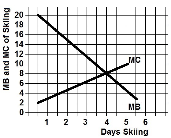
After studying this lesson you should be able to use Benefit Cost
Analysis (MB=MC) to answer this question.
1c Something Interesting - Why are we
studying this?
Drivers with airbags may take more risks
A similar question for skiers is why did the invention of avalanche airbags cause more people to become caught in avalanches (see below)? After studying this lesson you should be able to use Benefit Cost Analysis (MB=MC) to answer this question.
In a March 2013 blog post written by Utah Avalanche Center Director Bruce Tremper . . . Tremper says airbags are providing a false sense of security, leading more skiers into high-consequence terrain, and thus decreasing the effectiveness of said airbag."Each gizmo we buy to increase our safety usually cause us to increase our level of risk at the same time. For instance, when we added seat belts and airbags to cars, yes fatalities decreased, but it also allowed us to drive faster, farther, crazier and talk on our mobile phones at the same time. So safety measures usually work but not nearly as well as we would hope because people just increase their risk (and “utility”) at the same time. In avalanche airbag case, we will also get more powder, more fun, and more risk in the bargain . . . . people will increase their exposure to risk because of the perception of increased safety, which will cancel out some, but not all, of the effectiveness of avalanche airbag"What are avalanche airbags?
https://www.youtube.com/watch?v=h7QFRXc0R8M
Ch 1, pp. 11-20 (19th,10-21), "Society's Economizing Problem",
"Production Possibilities Model"
1c Assignments: Readings
Ch. 1, pp. 6-7 (19th p. 5), "Marginal Analysis: Comparing Benefits and Costs"
Ch. 1, pp. 14-15 (19th,13-14), "Optimal Allocation" (especially Fig 1.3),
Drivers with airbags may take more risks
Ch 1, p. 15 (19th, 14), "Consider This . . . The Economics of War"
PRODUCTION POSSIBILITIES
1c Assignments: Video
Lectures
1.4.1 Understanding the Concept of Production Possibilities Frontiers 24:46 [MyNotes]1.4.2 Understanding How a Change in Technology Affects the PPF 10:10 [MyNotes]
MAKING CHOICES: THE ECONOMIC WAY OF THINKING -- BENEFIT-COST ANALYSIS (also called Marginal Analysis or Cost-Benefit Analysis)
EconMovies- Episode 2: Monty Python and the Holy Grail - Marginal Analysis (YouTube ACDCLeadership 5:27)Thinking at the Margin (YouTube LearnLiberty 4:32) [MyNotes]
Incentives and Marginal Analysis (YouTube MrHurdleHistory 8:54) [MyNotes]
OTHER
Micro 1.1 The BIG Picture- AP Economics Overview (with links to playlists) (YouTube ACDCLeadership 12:49)ECONMOVIES Episode 3: Monsters Inc. and the Production Possibilities Curve
KEY PROBLEM
Using Benefit Cost Analysis (BCA)
http://www.harpercollege.edu/mhealy/eco211f/videos/1bprobbca.mp4
TOPICS
1c Outcomes - What you should
learn
- PPC (Production Possibilities Curve)
- BCA (Benefit Cost Analysis or Marginal Analysis)
OUTCOMES
Production Possibilities
- Construct a production possibilities curve (PPC) when given appropriate data; what is the production possibilities curve (PPC) or production possibilities frontier (PPF)?; what does it show?
- What are the assumptions behind the PPC
- Illustrate the following using the
production possibilities curve:
- we must make choices
- choices have opportunity costs
- the law of increasing costs
- the effect of unemployment
- the effect of productive inefficiency
- how present choices affect future possibilities
- the effect of international trade
- two types of "economic growth"
- it does NOT show the optimum product mix (allocative efficiency)
- Explain WHY the PPC has the shape that it does -- concave to the origin. What is the law of increasing cost?
- Why are there increasing costs? Why is the PPC concave to the origin? (Draw, Define. Describe all graphs)
- What would the PPC look like if there were constant costs?
- What does a point outside the PPC represent?
- What two things (2 Es) would a point inside the PPC indicate?
- Give some real-world applications of the production possibilities concept.
- Summarize the general relationship between investment and economic growth.
- What is the difference between "achieving the potential" and "increasing the potential"? Show the difference on a PPC. What are the two types of "economic growth" and how are they shown on a PPC?
- What would cause a PPC to shift inward?
- Use a PPC to illustrate the effect of international trade
- Be able to draw and explain the Circular Flow Model
Benefit Cost Analysis
- define benefit cost analysis (BCA) and use it to solve problems
- define "marginal" and give examples
- define marginal benefits (MB) and marginal costs (MC)
- explain why we ignore fixed, or sunk, costs ("Don't cry over spilt milk.")
- know what happens if MC increase? decrease?
- know what happens if MB increase? decrease?
- draw MB and MC on a graph and explain their shapes
- be able to find the optimum choice from a table of total costs and total benefits and from a table of marginal costs and marginal benefits
- use BCA to explain why Drivers with airbags may take more risks or why skiers with air bags may take more risks
- what is a "sunk cost" (or fixed cost) and why are they ignored when using benefit-cost analysis?
- "Don't cry over spilt milk " If you are deciding whether or not to come to class today, why does it not matter that you have already paid tuition? Why is the fact that you have paid tuition irrelevant when trying to decide whether to attend class today or skip?
Key
Terms Flash Cards - Click Here
1c Key Terms
Key Terms:
PPC:production possibilities, necessity of choice, law of increasing costs, concave to the origin, opportunity cost, constant cost, benefit cost analysis (marginal analysis), economic growth, consumer goods, capital goods, shrinking PPC, nonproportional growth
BCA:
marginal costs (MC), marginal benefits (MB), MB=MC Rule, sunk (fixed) costs
1c Key Problems
Production Possibilities Curve (PPC) - Click Here
Using Benefit Cost Analysis (BCA) - Click Here
Click here to see PPC questions
Using Benefit Cost Analysis (BCA) Question:
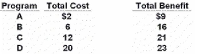
Use the above information on four different
highway programs of increasing scope to decide which program the
government should do.
All numbers are in billions of dollars.
Use Benefit Cost Analysis to answer the question.
MB = MC
1c Key Formulas
MB = change in Total Benefits / change in Quantity
MB = ![]() TB
/
TB
/ ![]() Q
Q
MC = change in Total Costs / change in Quantity
MC = ![]() TC
/
TC
/ ![]() Q
Q
Notice that I will use a triangle (![]() )
to mean "change in"
)
to mean "change in"
Production Possibilities Schedule and Curve
1c Key Graphs
PPC: Achieving Full Employment and Achieving
Productive Efficiency
(Achieving the Potential)
PPC: Economic Growth (Increasing the Potential)
Benefit Cost Analysis
1c Review
Quiz
- Production
Possibilities Curve- Econ 1.1
1c Review Videos
[3:56 YouTube ACDC Leadership]
- Shifting
the Production Possibilities Curve (PPC)- Econ
1.2
[5:35 YouTube ACDC Leadership]
NOTE: These are REVIEW videos only. In order to learn the material you must read the assigned textbook readings, watch the assigned lecture videos, and do problems. See the MACWEBAPP or the LESSONS link for these assignments.
Unit 1: Economics and
Globalization
Lesson 2a: Economic Systems and
Globalization
Because of scarcity we must make choices. An "economic system" is
the way that societies make economic choices. Because of scarcity all
countries must decide (1) what to produce, (2) how to produce, and
(3) who get what is being produced. Economic systems answer these
fundamental questions.
2a Introduction
All over the world economies are undergoing a process that I like to call "structural adjustment", but it is more commonly called "globalization". That is, countries are moving away from a command economy with government central planning to a laissez-faire market economy or capitalism. In this process the economic role of government is decreasing all over the world (well, almost).
In order to understand why this is happening we have to study unit 1, chapters 1, 2, 3 and 20, which are really MICROeconomic chapters. Strangely our Tomlinson videos do not discuss in depth the characteristics of market economies but our textbook does (chapter 2). Our textbook does not spend much time discussing command economies (planned economies), or economies in transition from planned to market (from command to capitalism), but the video lectures do!
When studying chapter 2, both the textbook and the videos, try to understand the following: (1) What are the characteristics of market and command economies? (2) What are their benefits and problems? and, (3) Why are countries moving away from a command economy toward a market economy?
In lesson 2a we will examine those questions. Then, in lesson 2b, we will look at what the role of government should play in a market economy. All over the world the economic role of government is decreasing, but it is not disappearing. So, what IS the economic role of government in market economies?
Structural adjustment, or globalization, has helped take nearly 1
billion people out of extreme poverty in 20 years. How? Read the
short article below.
2a Something Interesting - Why are we
studying this?
http://www.economist.com/news/leaders/21578665-nearly-1-billion-people-have-been-taken-out-extreme-poverty-20-years-world-should-aim/
In the fifth paragraph the article says:
"Most of the credit [for poverty reduction in the last twenty years] must go to capitalism and free trade, for they enable economies to grow - and it was growth principally that eased destitution."
We will take a look at the country of Venezuela which has the world's largest oil reserves and was once the richest country in South America. But now Venezuela has severe food and gasoline shortages and the world's highest inflation rate at over 15,000%. "[B]asic goods such as coffee, sugar, rice, milk, pasta, toilet paper, hand soap, and detergent remain impossible to find". Hospitals are without medicine, food is rationed, and people are fleeing the country. What happened? In the last two decades in order to help the poor, the government took control of the economy, nationalizing industries and controlling prices. And the economy has collapsed.
Online
2a Assignments: Readings
- A Comparison of Command Economies and Market Economies- Globalization and Structural Adjustment: http://www.economist.com/news/leaders/21578665-nearly-1-billion-people-have-been-taken-out-extreme-poverty-20-years-world-should-aim/
- Venezuela and Government Control of Economy: https://foreignpolicy.com/2016/06/19/venezuela-maduro-food-shortages-price-controls-political-unrest/
- OPTIONAL - Cuba Examines Asian Model For Economic Reforms (NPR Morning Edition)
Textbook:
Chapter 2 ALL (19th Ch. 2 ALL)Ch. 2, p. 47, (19th, 42), "Last Word: Shuffling the Deck"
Ch. 8, p. 186 (19th, 164), "Global Competition"
Chapter 23W of the 16th edition of our textbook, pages 2-13, found on our Blackboard site
- State Ownership and Central Planning: pp. 23W-2 to 23W-3
- Problems with Central Planning pp. 23W-3 to 23W-5
- The Collapse of the Soviet Economy pp. 23W-5 to 23W-6
- The Russian Transition to a Market System pp. 23W-6 to 23W-9
- Market Reforms in China pp. 23W-10 to 23W-11
- Outcome and Prospects pp. 23W-11 to 23W-13
- Conclusion pp. 23W-13
ECONOMIC SYSTEMS
2a Assignments: Video
Lectures
10.1.2 The Circular Flow Model 9:38 [MyNotes]1.1.4 An Overview of Economic Systems 10:50 [MyNotes]
Power of the Market (YouTube LibertyPen) 1:14 [MyNotes]
1.1.5 Case Study: The Work of Adam Smith 8:57 [MyNotes]
TRANSITION ECONOMIES
17.5.1 Centrally Planned Economies 10:57 [MyNotes]17.5.2 Policies to Change to Market Systems 11:18 [MyNotes]
17.5.3 Comparative Economic Performance 12:16 [MyNotes]
OPTIONAL (but interesting) Paul Solman Video: Capitalism vs. Socialism - The Cuban Quandary (YouTube PBS NewsHour) 13:56
GLOBALIZATION
Why Venezuela is in crisis CNN Money 1:49OPTIONAL: Economic Systems and Macroeconomics: Crash Course Economics #3 [10:18]
OPTIONAL: Globalization and Trade and Poverty: Crash Course Economics #16 [9:01]
TOPICS
2a Outcomes - What you should
learn
- Economic Systems
- Market Economies
- Command Economies
- Mixed Economies
- Structural Adjustment (Globalization)
- Characteristics of a Market Economy (Capitalism)
- Economics Systems and the 5Es
- Circular Flow Model
OUTCOMES
- What is "structural adjustment" and what are its policies and problems?
- Highlight the main features of a market economy and a command economy.
- List and explain the important characteristics of the American market system.
- Explain how a market system achieves
economic efficiency and why command economies do not.
- Describe how prices drive the movement of resources in a market system.
- The important role of profits and losses in a market economy
- Explain the role of self-interest and "invisible hand" in promoting economic efficiency.
- Explain why the command systems of the Soviet Union, Eastern Europe, and China failed.
- The coordination problem and incentive problem of command econmies
- What is the role of money in a market economy?
- "Between 1990 and 2010, the percent of people living in poverty fell by half as a share of the total population in developing countries, from 43% to 21%—a reduction of almost 1 billion people." WHY? What was the one main "poverty reduction measure" that contributed to this success? Explain.
- Understand some of the basic economic causes of the collapse (?) of the Venezuelan economy
- The circular flow model
Key
Terms Flash Cards - Click Here
2a Key Terms
Key Terms:
structural adjustment, economic system, command system (centrally planned, socialism, command economy), market system (captialism, laissez-faire, market economy), mixed economic system, Bolshevik revolution, self interest, private property, freedom of enterprise and choice, competition, market, specialization, consumer sovereignty, dollar votes, invisible hand, creative destruction, coordination problem, incentive problem, circular flow diagram, product market, resource market, privatization, nationalization, central planning, shock therapy, import substitution
2a Key Graphs
World Decrease in Poverty - mostly caused by Structural Adjustment
Circular Flow Model
2a Review Quizzes: Capitalism
/ Command
Economies
- Econ
1.6- Economic Systems: Why is Communist China doing so
well?
2a Review Videos
[4:13 YouTube ACDC Leadership]
NOTE: These are REVIEW videos only. In order to learn the material you must read the assigned textbook readings, watch the assigned lecture videos, and do problems. See the MACWEBAPP or the LESSONS link for these assignments.
Unit 1: Economics and
Globalization
Lesson 2b: The Economic Role of
Government and Government Finance
Now, you should have a good idea of the characteristics, benefits,
and problems of the two main types of economic systems and understand
how, and why, countries seem to be moving toward a market, or more
laissez-faire, system. Here we will examine the economic functions of
government in a market economy.
2b Introduction
Most economists, and politicians, agree on these general principles, BUT they may disagree strongly on the degree of involvement the government should have in the economy. I think, most people agree on WHAT the government should do, but they disagree on HOW MUCH.
We learned in lesson 2a that market economies are efficient and that centrally (government) planned command economies are inefficient. So whenever there is government involvement in a market economy we should ask WHY? If market economies are efficient and efficiency reduces scarcity, why would the government get involved? We will learn that sometimes the government is needed to ASSIST a market economy to be efficient and sometimes a market economy is inefficient and the government is needed to FIX it.
After looking at the economic functions of government we will look at government finance in the United States. Latter in this course we will discuss how the goverment uses spending and taxation to affect the economy. Here we learn what the government spends its money on and where governments get their revenue (taxes).
Skim the news articles below about raising taxes on gasoline and
putting taxes on soda and junk food. After studying this lesson you
should understand why many people support these taxes.
2b Something Interesting - Why are we
studying this?
Why might
gasoline prices be too low?
http://www.npr.org/templates/story/story.php?storyId=4858826
Why are several cities and states considering a tax on sodas?
http://www.stltoday.com/news/local/illinois/buying-soft-drinks-in-illinois-would-cost-more-under-tax/article_5eccc299-6c48-5b44-9643-95bce5365dee.htmlhttp://www.sfgate.com/bayarea/article/Tax-on-soda-to-be-floated-in-San-Francisco-4932025.php
Why did Mexico tax junk food and soda?
http://www.politico.com/story/2014/01/mexico-soda-tax-101645
Economic
Functions of Goverment
2b Assignments: Readings
Ch. 4, pp. 90-94, 96-100, (19th, 99-102, 104-108) "Public Goods", "Externalities"
Microeconomics Chapter 16 (found on our Blackboard site): pp 338-346
- Government Finance;
- Federal Finance;
- State and Local Finance;
- Local, State, and Federal Employment;
- Apportioning the Tax Burden;
- The VAT
Tax Brackets (Marginal Tax Rates) (audio or reading only)
Role
of Government in a Mixed Economy
(YouTube - Daniel Mares15:53) [MyNotes]
2b Assignments: Video
Lectures
When is a Potato Chip Not Just a Potato Chip (YouTube-LearnLiberty 4:46)
Public Goods and Asteroid Protection (MRUniversity 2:30)
EconMovies 7: Anchorman (Efficiency and Market Failures)
A Deeper Look at Public Goods (MRUniversity 7:55)
Where do your tax dollars go? (YouTube - Test Tube News 3:44)
8.2.2 Analyzing the Tax System (8:19) [MyNotes]
OPTIONAL: Tax Brackets and Progressive Taxation Khan Academy (4:14)
TOPICS
2b Outcomes - What you should
learn
- Economic Functions of Government in an Market Economy
- Government Finance:
- Expenditures and Revenues
- Average and Marginal Tax Rates
- Progressive, Proportional, and Regressive taxes
OUTCOMES
- Functions of Government
- Understand the five functions of government in a market economy
- stabilization policies: what should the government do if unemployment is high? if inflation is high?
- Negative Externality:
- too much produced without government, why?
- government micht tax or regulate to reduce consumption
- Positve Externality:
- Too little produced without government, why?
- government might subsidize or produce the product itself to increase production
- Public good
- nonexcludable and nonrival
- NONE produced without government
- government must produce
- Why are public schools, public parks, and public libraries NOT "public goods"?
- Government Finance
- What are the major revenue sources and major expenditures for the federal, state, and local governments?
- Define and give examples of progressive, proportional, and regressive taxes.
- Be able to calculate average tax rates, marginal tax rates, and taxes paid
- Calculate average tax rates and marginal tax rates.
- What are the PROS and CONS of using a lottery to finance government?
- Discuss the progressivity or
regressivity of the following taxes:
- federal income tax
- sales tax
- payroll tax (Social Security Tax)
- property tax
- exhaustive and non exhaustive government
purchases
or government purchases vs. government spending, - benefits received principle, vs. ability-to-pay principle (sometimes called the equal sacrifice principle) and the law of diminishing marginal utility
Key
Terms Flash Cards - Role of Government - Click Here
2b Key Terms
Key Terms Flash Cards - Government Finance - Click Here
Key Terms:
Role of Government:consumer sovereignty, monopoly, natural monopoly, antitrust, transfer payments, market intervention, market failure, negative externality, positive externality, public goods, private goods, rivalry, nonrival, excludability, nonexcludability, free-rider problem, macroeconomic stability, fiscal policy, monetary policy, expansionary fiscal policy, easy money policy, contractionary fiscal policy, tight money policy,Government Finance:
government purchases, exhaustive, transfer payment, nonexhaustive, deficit spending, personal income tax, payroll tax, benefits received principle, ability-to-pay principle, average tax rates, marginal tax rates, progressive tax, proportional tax, regressive tax, value added tax (VAT)
Calculate
tax owed, marginal tax rate, and average tax rate
2b Key Problems
If Taxable Income is Between:
The Tax Due is:
Given the Tax Rate Schedule above, calculate the following:
If taxable income is
$9,325: The amount of tax owed:
__________________ The marginal tax rate:
__________________ The average tax rate:
__________________ If taxable income is
$10,325: The amount of tax owed:
__________________ The marginal tax rate:
__________________ The average tax rate:
__________________
2b Key Formulas
Average Tax Rate = taxes paid / income
Marginal Tax Rate = change in taxes paid / change in income
Marginal Tax Rate = ![]() taxes /
taxes / ![]() income
income
Notice that I will use a triangle (![]() )
to signify "change in"
)
to signify "change in"
2b Review Quizzes: Market
Failures / Gov't
Finance
Micro
Unit 6 Intro- Market Failures and the Government
2b Review Videos
[2:31 YouTube ACDC Leadership]
NOTE: These are REVIEW videos only. In order to learn the material you must read the assigned textbook readings, watch the assigned lecture videos, and do problems. See the MACWEBAPP or the LESSONS link for these assignments.
Unit 1: Economics and
Globalization
Lesson 3a: Demand
If the price of pizza goes up, what happens to the demand for pizza?
. . . . . . . . . . . . . . . . .
. . . . . . . . . . . . .
3a Introduction
The next three lessons introduce the demand and supply model for explaining how prices arise and change in a market economy. Learn these lessons well. Do the assigned problems. Draw the graphs in the Yellow Pages and while you are reading and studying. DRAW GRAPHS! Get used to using the graphs to help you answer questions. If you are avoiding drawing the graphs you will do poorly and not get the practice that you need to learn the concept.
So why doesn't the demand for pizza change if the price changes? Because economists have a different definition of "demand". Demand is NOT the quantity that we buy. If the price of pizza goes up we will buy less, but that is not what "demand" means in economics.
Economists tend to be precise with their definitions and sometimes their definitions are different than the more commonly used definitions. Things like "scarcity", "investment", "cost", "demand", and "supply", have different definitions in economics than what you may already know. Learn our definitions! Demand is not how much we buy. Demand has a different definition in economics. "Demand" means the "demand graph".
Economists use models (like the supply and demand model) to simplify the real world. They do this by isolating certain variables from all the clutter found in reality. Then by changing one variable at a time economists can see what effect it will have.
In this lesson we will learn the economic definition of DEMAND and plot the demand graph. Then, we will look at one variable at a time to see what effect they have on the demand curve. We call these variables the "non-price determinants of demand". They are: Pe, Pog, I, Npot, T or "PPINT". LEARN THEM! LEARN THEM WELL! Know how each one affects the demand curve. Be sure to do the Yellow Pages and other Practice Activities until you understand the concept well.
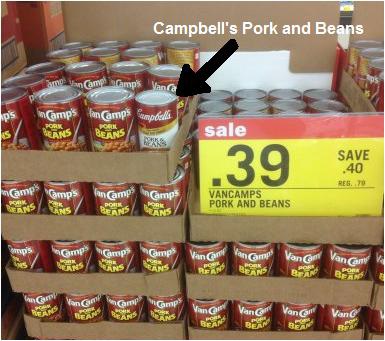
See the picture below. VanCamp's Pork and Beans are on sale (price
is lower). Notice that there is a can of Campbell's Pork and Beans on
the sale display.
3a Something Interesting - Why are we
studying this?
What is that Campbell's Pork and Beans can doing on the display for VanCamp's Pork and Beans?
After studying this lesson you will be able to draw a graph illustrating what happened to the demand for Campbell's Pork and Beans when a customer took a can out of their shopping cart and placed it on this display of VanCamp's beans that were on sale.
Ch 3, pp. 53-59, (19th 47-53) "Demand"
3a Assignments: Readings
2.1.1 Understanding
the Determinants of Demand 11:58
[MyNotes]
3a Assignments: Video
Lectures
2.1.2 Understanding the Basics of Demand 11:54 [MyNotes]
2.1.3 Analyzing Shifts in the Demand Curve 8:13 [MyNotes]
2.1.4 Changing Other Demand Variables 10:43 [MyNotes]
2.1.5 Deriving a Market Demand Curve 9:16 [MyNotes]
OPTIONAL:
The Law of Demand (econclassroom.com 11:24)Changes in Demand versus Changes in Quantity Demanded (econclassroom.com 5:52)
The Determinants of Demand (econclassroom.com 11:07)
TOPICS
3a Outcomes - What you should
learn
- Demand:
- Define
- Draw
- Describe
- Determinants
OUTCOMES
- define demand (note: it has a DIFFERENT DEFINITION in economics)
- If the price of pizza goes up, why does the demand for pizza stay the same?
- be able to correctly draw and label a demand graph
- why do economists employ the ceteris paribus assumption when creating a demand curve?
- what is the law of demand?
- why is the demand curve downward sloping (three explanations)
- list the non-price determinants of demand (Pe. Pog, I, Npot, T) and understand how they affect the demand schedule and curve. This is VERY IMPORTANT. BE ABLE TO DO THIS! See the 3a/3b/3c yellow pages.
- explain the difference between the a "change in the quantity demanded" and a "change in demand"
- what is an increase in demand and a decrease in demand and show how they affect the demand schedule and the demand curve
- what is "market demand"?
- what is that Campbell's Pork and Beans can doing on the display for VanCamp's Pork and Beans (see picture at left)? Which non-price determinant of demand explains why that Campbell's soup can is there?
3a Non-Price Determinants of Demand and Supply |
Pe -- expected price
Pog -- price of other goods1) substitute goods
2) complementary goods
3) independent goodsI -- income
1) normal goods
2) inferior goodsN -- number of POTENTIAL consumers
T -- tastes and preferences
Non-Price Determinants of Supply (PPPTTN)
Pe -- expected price
Pog -- price of other goods produced by same firm
Pres -- price of resources
T --technology
T --taxes and subsidies
N -- number of producers/sellers
NON-PRICE DETERMINANTS OF DEMAND
Pe -- expected price
Pe in the future

Pe in the future
Pog -- price of other goods
1) substitute goods
2) complementary goods
I -- income
1) normal goods
2) inferior goods
Npot -- number of POTENTIAL consumers
T -- tastes and preferences
NON-PRICE DETERMINANTS OF SUPPLY
Pe -- expected price
Pog -- price of other goods also produced by the same firm
Pres -- price of resources
Tech --technology
Improved technology
Tax --taxes and subsidies
N -- number of producers/sellers
Key
Terms Flash Cards - Click Here
3a Key Terms
Key Terms:
demand, quantity demanded, law of demand, market demand, horizontal summation, income effect, substituion effect, diminishing marginal utility, change in demand, change in quantity demanded, increase in demand, decrease in demand, non-price determinants of demand, normal good, inferior good, substitute good, complementary good (complement), independent goods
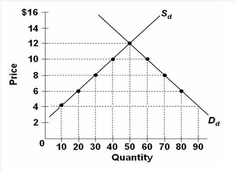
Demand Schedule and Curve
3a Key Graphs
Change in Quantity Demanded
Change in Demand: Increase
Change in Demand: Decrease
Market Demand
- Demand
and Supply Explained- Econ 2.1
3a Review Videos
[6:20 YouTube ACDC Leadership]
NOTE: These are REVIEW videos only. In order to learn the material you must read the assigned textbook readings, watch the assigned lecture videos, and do problems. See the MACWEBAPP or the LESSONS link for these assignments. .
Unit 1: Economics and
Globalization
Lesson 3b: Supply
If the price of pizza goes up what happens to the SUPPLY of pizza?
NOTHING!
3b Introduction
A change in the price of a product does not affect its supply, or its demand. When the price goes up the QUANTITY SUPPLIED will increase, but the supply does not change. Learn the difference between "supply" and "quantity supplied". "Supply" does NOT MEAN the quantity available for sale. Supply has a different definition in economics. "Supply" means the "Supply graph".
So what would cause the supply graph, or supply itself, to change? Those things that cause supply to change are called the "non-price determinants of supply". They are: Pe, Pog, Pres, Tech, Tax, Nprod or "PPPTTN". See the Yellow Pages.
Remember, the goal of chapter 3 is to learn a model that will help us understand why prices are what they are and why they change. In the next lesson we will put demand and supply together and use the model (graph) to find the prices of products. Then, and more importantly, we will see what causes prices to change.
After completing this chapter, if you hear on the news, or read in your news app, that the price of gasoline is going down, we will be able to explain WHY. The causes of changes in prices of products are the five non-price determinants of demand (Pe, Pog, I, Npot, T) and/or the six non-price determinants of supply (Pe, Pog, Pres, Tech, Tax, Nprod.). Whenever you hear that the price of something is changing think of these 11 possible causes.
Read the short news article below on the declining price of gasoline
(Dec. 2015). Paragraph 10 states "Plunging oil prices are the main
factor driving down the price at the pump. "
3b Something Interesting - Why are we
studying this?
After studying this lesson you should be able to (1) list the non-price determinants of supply, (2) select the determinant that is the cause of the decline in gasoline prices discussed in the news article above, and (3) graph the effect that the change in the determinant will have on the supply curve for gasoline.
Ch. 3, pp. 59-62, (19th, 53-56) "Supply"
3b Assignments: Readings
Where
Is All That Excess Oil Going?
[Why are they storing oil? What is happening to supply? Which
determinant has caused the supply to change?]
Read this online lecture: Demand and Supply
2.2.1 Understanding
the Determinants of Supply 7:25
[MyNotes]
3b Assignments: Video
Lectures
2.2.2 Deriving a Supply Curve 9:49 [MyNotes]
2.2.3 Understanding a Change in Supply versus a Change in Quantity Supplied 6:52 [MyNotes]
2.2.4 Analyzing Changes in Other Supply Variables 8:47 [MyNotes]
2.2.5 Deriving a Market Supply Curve from Individual Supply Curves 7:16 [MyNotes]
OPTIONAL
AC Econ 2.2 Demand and Supply Explained (2 of 2) (4:54 but just watch up to 2:45)EP AP Macro-Economics - Determinants of Supply [YouTube - ExamPop]
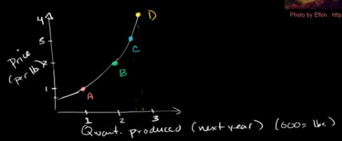
KA Factors affecting supply (6:57) NOTE : It looks like the supply graph is labelled "D", but that is just point D (A, B, C, D) on the supply curve.
TOPICS
3b Outcomes - What you should
learn
- Supply
- Define
- Draw
- Describe
- Determinants
OUTCOMES
- define supply (note: it has a DIFFERENT DEFINITION in economics)
- be able to correctly draw and label a supply graph
- if the price of pizza goes up why does the supply not change?
- why do economists employ the ceteris paribus assumption when creating a supply curve?
- what is the law of supply?
- why is the supply curve upward sloping (two explanations)
- list the non-price determinants of supply (Pe, Pog, Pres, Tech, Taxes, Nprod) and understand how they affect the supply schedule and curve. This is VERY IMPORTANT. BE ABLE TO DO THIS! See the 3a/3b/3c yellow pages.
- explain the difference between the a "change in the quantity supplied" and a "change in supply"
- what is an increase in supply and a decrease in supply and show how they affect the supply schedule and the supply curve
- what is "market supply"?
- Read the following and answer these
questions:
- Which determinant has changed?
- Will it affect S or D of gasoline?
- Will the S or D of gasoline increase or
decrease? Shift to the right or to the left?
"According to the Lundberg Survey, the average price for regular gasoline dropped 3.99 cents over the three weeks up to July 11 to $3.6699 per gallon. . . . Lundberg explained that the average gasoline price continues to decrease because refiners, enjoying the lower crude oil prices in the market, are passing down the savings to the consumers. "
3b Non-Price Determinants of Demand and Supply |
Pe -- expected price
Pog -- price of other goods1) substitute goods
2) complementary goods
3) independent goodsI -- income
1) normal goods
2) inferior goodsN -- number of POTENTIAL consumers
T -- tastes and preferences
Non-Price Determinants of Supply (PPPTTN)
Pe -- expected price
Pog -- price of other goods produced by same firm
Pres -- price of resources
T --technology
T --taxes and subsidies
N -- number of producers/sellers
NON-PRICE DETERMINANTS OF DEMAND
Pe -- expected price
Pog -- price of other goods
1) substitute goods
2) complementary goods
I -- income
1) normal goods
2) inferior goods
Npot -- number of POTENTIAL consumers
T -- tastes and preferences
NON-PRICE DETERMINANTS OF SUPPLY
Pe -- expected price
Pog -- price of other goods also produced by the same firm
Pres -- price of resources
Tech --technology
Improved technology
Tax --taxes and subsidies
N -- number of producers/sellers
Key
Terms Flash Cards - Click Here
3b Key Terms
Key Terms:
supply, quantity supplied, market supply, horizontal summation, law of supply, change in supply, change in quantity supplied, increase in supply, decrease in supply, non-price determinants of supply
Supply Table and Curve
3b Key Graphs
Increase in Supply
Decrease in Supply

- Demand
and Supply Explained (2 of 2) - Econ 2.2
3b Review Videos
[4:54 YouTube ACDC Leadership]
NOTE: These are REVIEW videos only. In order to learn the material you must read the assigned textbook readings, watch the assigned lecture videos, and do problems. See the MACWEBAPP or the LESSONS link for these assignments.
Unit 1: Economics and
Globalization
Lesson 3c: Market Equilibrium
and Efficiency - So, what happens to Price and
Quantity?
We are going to learn two very important things in this
lesson.
3c Introduction
First, we will put demand and supply together and learn how to use the model to to see why products have the prices that they do. Then, and more importantly, we will see what causes prices to change.
If you hear on the news or read in your news app, that the price of gasoline is going down, we will be able to explain WHY. The causes of changes in prices of products are the five non-price determinants of demand (Pe, Pog, I, Npot, T) and/or the six non-price determinants of supply (Pe, Pog, Pres, Tech, Tax, Nprod.). Whenever you hear that the price of something is changing think of which of these 11 possible causes have changed, draw the graph and shift the appropriate demand and/or supply graph, and the graph will show the price changing.
Second, after we learn that in a competitive market economy the interaction of demand and supply will determine what the prices of products will be and how much people will buy at that price, we will ask: Is this the allocatively efficient quantity and price? Our goal is to show that in a competitive market the price will change until allocative efficiency is achieved. In chapter 2 we learned that markets are allocatively efficient. This means they will produce the quantity of goods that maximizes the society's satisfaction. After studying chapter 3 we will bew able to show the allocatively efficient price and quantity on a graph.
Competitive markets are efficient.
Read the first few paragraphs of Hybrid
Car Prices Increasing Due To High Gas Prices.
3c Something Interesting - Why are we
studying this?
In lesson 3a you learned how the non-price determinants of demand (Pe, Pog, I, N, T) affect the demand curve. In lesson 3b you learned how the non-price determinants of supply (Pe, Pog, Pres, Tech, Tax, Nprod) affect the supply curve.
After studying this lesson you will be able to use these determinants and graphs to explain why prices change. For example you will understand why: "It's becoming almost an annual tradition: As fuel prices rise in the spring, so do the prices of hybrid cars. "
Ch. 3, pp. 62-70, 75-80, (19th, 56-64, 69-74), "Market Equilibrium",
"Additional Examples of Supply and Demand"
3c Assignments: Readings
Ch. 4, pp. 85- 90, (19th, 93-99), "Efficiently Functioning Markets"
Supply, Demand, and Economic Efficiency
PUTTING SUPPLY AND DEMAND TOGETHER
3c Assignments: Video
Lectures
2.3.1 Determining a Competitive Equilibrium 11:04 [MyNotes]2.3.2 Defining Comparative Statics 7:02 [MyNotes]
2.3.3 Classifying Comparative Statics 11:54 [MyNotes]
AC Micro 2.4 Double Shifts in Supply and Demand: Econ Concepts in 60 Seconds (2:34)
EconMovies: Episode 4: Indiana Jones (Demand, Supply, Equilibrium, Shifts) (7:02)
MARKETS AND EFFICIENCY
Efficiency and Equilibrium in Competitive Markets (econclassroom.com 11:48) [begin at 7:27 and stop at 8:44, we will not cover consumer and producer surplus] [MyNotes]
TOPICS
3c Outcomes - What you should
learn
- Market Equilibrium
- Market Equilibrium and Changes in D and S
- Market Equilibrium and Allocative Efficiency
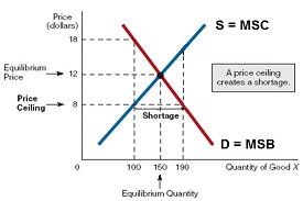
- Price Ceilings, Price Floors, and Allocative Efficiency
OUTCOMES
Market Equilibrium
- Explain the concept of equilibrium price and quantity.; define equilibrium; find the equilibrium price and quantity on a supply and demand schedule and graph
- Illustrate graphically equilibrium price and quantity.
- what happens if the price is below the equilibrium price? If it is above it?
- define "shortage" and "surplus" and explain using a supply and demand graph
- the four steps to finding a new equilibrium when a non-price determinant changes and how to use them (see the yellow pages)
- what happens to the equilibrium price and quantity if (1) demand increases, (2) demand decreases, (3) supply increases, and (4) supply decreases.
- Explain and graph the effects of simultaneous changes in demand and supply on equilibrium price and quantity
- Price ceilings, price floors, and allocative efficiency
Markets and Efficiency
- define marginal social benefit and explain why it is often measured by the demand curve
- define marginal social cost and explain why it is often measured by the supply curve
- explain why allocative inefficiency occurs where MSB > MSC causing an underallocation of resources; show on graph using the MSB=MSC model
- explain why allocative inefficiency occurs where MSB < MSC causing an overallocation of resources; show on graph using the MSB=MSC model
- Explain how equilibrium achieves allocative efficiency.
- be able to find WHAT WE GET and WHAT WE WANT the MSB=MSC model graph
3c Non-Price Determinants of Demand and Supply |
Pe -- expected price
Pog -- price of other goods1) substitute goods
2) complementary goods
3) independent goodsI -- income
1) normal goods
2) inferior goodsN -- number of POTENTIAL consumers
T -- tastes and preferences
Non-Price Determinants of Supply (PPPTTN)
Pe -- expected price
Pog -- price of other goods produced by same firm
Pres -- price of resources
T --technology
T --taxes and subsidies
N -- number of producers/sellers
NON-PRICE DETERMINANTS OF DEMAND
Pe -- expected price
Pog -- price of other goods
1) substitute goods
2) complementary goods
I -- income
1) normal goods
2) inferior goods
Npot -- number of POTENTIAL consumers
T -- tastes and preferences
NON-PRICE DETERMINANTS OF SUPPLY
Pe -- expected price
Pog -- price of other goods also produced by the same firm
Pres -- price of resources
Tech --technology
Improved technology
Tax --taxes and subsidies
N -- number of producers/sellers
Key
Terms Flash Cards - Click Here
3c Key Terms
Key Terms:
equilibrium, market equilibrium, bidding mechanism, surplus, shortage, scalping, productive efficiency, allocative efficiency, marginal social benefits, marginal social costs, "what we get", "what we want", profit maximizing quantity, underallocation of resources, overallocation of resources, price ceiling, price floor
3c Key Problems
Click on the links above to learn how to use a supply and demand graph to show why prices and quantities change. The exam 1 extra credit question will be similar to these problems.
Use the four-step process to explain what happens to PRICE (P) and QUANTITY (Q) of the following goods using the information provided in the short news articles below.
Four Step Process1. Which determinant has changed?
2. Will it affect Supply (S) or Demand (D)?
3. Will S or D increase or decrease?
4. GRAPH IT and show what happens to P and Q.Non--Price Determinants of Demand (PPINT)
Pe -- expected price
Pog -- price of other goods (subs and Complw)
I - income (normal and inferior goods)
N -- number of POTENTIAL consumers
T -- tastes and preferencesNon-Price Determinants of Supply (PPPTTN)
Pe -- expected price
Pog -- price of other goods PRODUCED. BY THE SAME FIRM
Pres -- price of resources
T - technology of production
T -- taxes and subsidies
N -- number of sellersProduct: Beef. What happens to P and Q? Circle and label determinants. Show effects on a graph.
http://www.bloomberg.com/news/articles/2014-11-18/us-beef-supply-will-fall-again-in-2015-chicken-demand-will-riseDomestic beef production has been waning [decreasing] for years because of rising feed and energy prices. A drought in 2012 caused feed prices to spike and, in response, farmers thinned their herds.Product: Chicken. What happens to P and Q? Circle and label determinants. Show effects on a graph.
http://www.bloomberg.com/news/articles/2014-11-18/us-beef-supply-will-fall-again-in-2015-chicken-demand-will-riseIt's been an expensive year to eat beef, and 2015 doesn't look any cheaper. . . . Consumers have traded down to less expensive meats such as chicken.Product: Almonds. What happens to P and Q? Circle and label determinants. Show effects on a graph.
http://www.cnbc.com/2016/08/29/california-almond-harvest-may-break-records-despite-drought.htmlWith the drought easing in parts of California, this year's almond harvest is shaping up to be a record haul …. Consumers have already taken an interest in almond products because of their "heart health" benefits.Product: McDonald's meals. What happens to P and Q? Circle and label determinants. Show effects on a graph.
http://www.bloomberg.com/news/articles/2014-10-20/mcdonald-s-costly-burgers-send-diners-to-fancier-rivalsMike Hiner used to take his grandsons to McDonald's when they wanted a treat. With higher wage and food costs pushing up prices at the Golden Arches, he's increasingly taking them to IHOP, Denny's and Chili's instead . . . . The chain's diminishing appeal among budget diners -- coupled with rising meat costs -- are projected to take a bite out of third-quarter earnings due to be reported tomorrow.
.
Market Equilibrium
3c Key Graphs
Changes in Demand And Supply
Price Ceiling
Price Floor

3c Review
Quiz - Lessons 3a, 3b, and 3c
- Shifting
Demand and Supply- Econ 2.3
3c Review Videos
[4:49 YouTube ACDC Leadership]
- Double
Shifts- Econ 2.5 (Technical Tuesday)
[3:26 YouTube ACDC Leadership]
- Price
Ceilings and Floors- Economics 2.6
[4:34 YouTube ACDC Leadership]
NOTE: These are REVIEW videos only. In order to learn the material you must read the assigned textbook readings, watch the assigned lecture videos, and do problems. See the MACWEBAPP or the LESSONS link for these assignments.
Unit 1: Economics and
Globalization
Lesson 20a: Why we Trade: Comparative
Advantage
In Lesson 2a we learned about the following Structural Adjustment
Policies and the following characteristics of capitalist
economies:
20a Introduction
Structural Adjustment Policies:
- Privatization
- Promotion of Competition
- Reduced Role of Government
- Removing Price Controls
- FREER TRADE and Convertible Currency
- Foreign Investment
Characteristics of Capitalist
Economies:
- private property
- freedom of enterprise and choice
- role of self interest
- competition -
- markets and prices
- limited role for government
In this lesson we will study trade.Trade increases competition and helps the world's economies achieve PRODUCTIVE EFFICIENCY (producing at a minimum cost by using resources where they are best suited). Therefore it is an important concept to study in any introductory economics course.
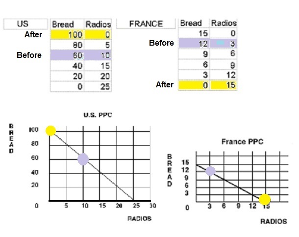
We will learn that trade based on COMPARATIVE ADVANTAGE can help the world PRODUCE MORE from the same amount of resources. Trade allows all countries to consume beyond their production possibilities (point E on the graph below).
How is that possible?
We will also learn that even if a country is better at producing all products, it is still possible for it to come out ahead if it specializes and trades with other (less productive) countries.
How is that possible?
That is why there has been a trend over several decades of the world moving to ward freer and freer trade.
Read the first four paragraphs of The
Mystical Power of Free Trade.
20a Something Interesting - Why are
we studying this?
After studying this lesson you should understand:
- why "society benefits from allowing its citizens to buy what they wish--even from foreigners." (i.e. the gains from trade),- and why "people resist this conclusion, sometimes violently"
Ch. 20, pp. 442-452 (19th, 398-407), "Some Key Trade Facts", "The
Economic Basis for Trade", "Comparative Advantage"
20a Assignments: Readings
"The Mystical Power of Free
Trade"
http://www.cnn.com/ALLPOLITICS/time/1999/12/06/free.trade.html
VERY USEFUL: Lecture Outline
1.5.1 Defining
Comparative Advantage with the Production Possibilities
Frontier 22:10 [MyNotes]
20a Assignments: Video
Lectures
1.5.2 Understanding Why Specialization Increases Total Output 6:46 [MyNotes]
1.5.3 Analyzing International Trade Using Comparative Advantage 25:35 [MyNotes]
1.5.4 Outsourcing 8:54 [MyNotes]
17.4.3 Hot Topic: Winners and Losers in NAFTA 4:20 [MyNotes]
KEY PROBLEM: The gains from trade
OPTIONAL
KA Comparative advantage specialization and gains from trade (8:55)EC Determining Comparative Advantage using PPCs – Worked solutions to AP Free Response Questions (8:27)
TOPICS
20a Outcomes - What you should
learn
- Why do we trade?
- Absolute Advantage, Comparative Advantage, and the Gains from Trade
- Terms of Trade
OUTCOMES
- why do the gains from trade appear to be hidden from many people?
- what is the economic basis for specialization and exchange (trade)?
- calculate the opportunity costs using straight line production possibilities
- define and find absolute advantage and comparative advantage using straight line (constant costs) production possibilities
- calculate how specialization and trade increases output using the production possibilities tables or graphs of two different countries (i.e. calculate the gains from trade)
- compute the minimum and maximum terms of trade
Key
Terms Flash Cards - Click Here
20a Key Terms
Key Terms:
opportunity cost, constant costs, increasing costs, absolute advantage, comparative advantage, gains from trade, free trade, terms of trade, minimum and maximum terms of trade
20a Key Problems
The Gains from Trade - Click Here
Click on the link above to learn how to do this problem.
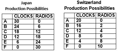
Assume that prior to specialization and trade, Japan produced at point D and Switzerland produced at point E. Calculate the possible gains from specialization and trade.
Comparative Advantage and the Gains from Trade
20a Key Graphs
20a Review
Quiz
- Comparative
advantage specialization and gains from trade | Microeconomics | Khan
Academy
20a Review Videos
[8:55 YouTube Khan Academy]
NOTE: These are REVIEW videos only. In order to learn the material you must read the assigned textbook readings, watch the assigned lecture videos, and do problems. See the MACWEBAPP or the LESSONS link for these assignments.
Unit 1: Economics and
Globalization
Lesson 20b: International Trade and
Foreign Exchange Markets
Everything discussed in Lesson 20a about trade (specialization and
exchange) can be applied to trade between individuals, cities,
counties, states, and countries. In this lesson we will focus
specifically on INTERNATIONAL trade (trade between countries).
20b Introduction
Comparative advantage still applies, but there are some differences between INTERnational trade (trade between countries) and INTRAnational trade (trade within a country). These differences include greater distances, politics, and the use of different currencies.
Lesson 20b begins with a review of the FACTS of international trade (see: Lecture Outline). Then we will look at what happens when politicians restrict trade (and therefore cause inefficiency). And we will finish up with learning how to use a supply and demand graph to understand why exchange rates change.
Concerning exchange rates: students often believe that a strong dollar is good and a weak dollar is bad. This is not always true. If the U.S. dollar appreciates (increases in value) it is often called a "strong dollar". What a strong dollar does is make it cheaper for Americans to buy foreign imports (or make it cheaper to take a ski trip in Canada). A strong dollar also makes it more expensive for foreigners to purchase U.S. exports. Therefore, a strong dollar may be good for consumers because of cheap imports, but bad for workers because of less exports, fewer jobs, and more unemployment).
The link below goes to a LIST of articles on the international
trade agreements, including the Trans Pacific Partnership (TPP),
found on the Huffington Post news site. President Trump took the US
out of the TPP soon after he became president. The Huffington Post
tends to be a more liberal news site, that is less supportive of free
trade. Scroll down just looking at the titles of the news
articles over the last few months. You will see that many of them
appear to oppose the free trade agreements.
20b Something Interesting - Why are
we studying this?
Trans
Pacific Partnership
http://www.huffingtonpost.com/news/trans-pacific-partnership/
After studying this lesson you will have a better understanding of why many people oppose such trade agreements BUT most economists say that such agreements benefit the US economy and the world economy.
Ch. 20, pp. 443-465 (19th, 398-418), "Some Key Trade Facts", "Trade
Barriers and Export Subsidies", "The Case for Protection",
"Multilateral Trade Agreements and Free-Trade Zones"
20b Assignments: Readings
Ch. 20, p. 464 (19th, 419), "The Last Word - Petition of the Candlemakers, 1845"
Ch. 21, 475-78 (19th, 429-432), "Flexible Exchange Rates"
Ch. 21, 484-488 (19th, 438-439) "Recent U.S. Trade Deficits"
Trans-Pacific Partnership
- http://www.nytimes.com/2015/05/12/business/unpacking-the-trans-pacific-partnership-trade-deal.html
VERY USEFUL: Lecture Outline
17.4.2 Trade
Policy 7:17 [MyNotes]
20b Assignments: Video
Lectures
17.1.1 Determining the Difference between a Closed Economy and an Open Economy 8:55 [MyNotes]
Why do Countries Restrict Trade? (8:34) [MyNotes]
Types of Trade Restrictions (9:43) [MyNotes]
17.1.2 Understanding Exports in an Open Economy 5:22 [MyNotes]
17.3.1 Nominal Exchange Rates 11:32 [MyNotes]
17.3.4 Determination of Exchange Rates 12:31 [MyNotes]
17.3.5 Floating and Fixed Systems 13:18 [MyNotes]
TOPICS
20b Outcomes - What you should
learn
- Facts About Trade
- Trade Restrictions
- Exchange Rates
- Trade Deficits
OUTCOMES
- summarize the importance of international trade to the U.S. in terms of overall volume and major trading partners.
- list the major imports and exports of the United States and identify the major its major trading partners
- identify types of trade barriers
- describe the economic impact of tariffs, including both direct and indirect effects.
- contrast the economic impact of a quota with that of a tariff.
- list six arguments in favor of protectionist barriers, and critically evaluate each
- who gains from trade restrictions? who loses?
- the two most popular arguments against free trade are (1) we need to restrict trade to crease more jobs here, and (2) how can our workers compete against workers who are paid only a few dollars a day? Why do these two argments make NO ECONOMIC SENSE?
- why are import quotas more restrictive than tarriffs?
- identify the costs of protectionist policies and their effects on income distribution.
- understand the benefits and problems of a "strong dollar" and a "weak dollar"
- what causes exchange rates to appreciate and depreciate?
- understand the causes and effects of trade deficits
Key
Terms Flash Cards - Click Here
20b Key Terms
Key Terms:
imports, exports, trade barriers, tariff, revenue tariff, protective tariff, import quota, nontariff barrier, export subsidies, special interest effect, infant industry, dumping, WTO, NAFTA, TPP, offshoring, exchange rate, strong dollar, weak dollar, appreciation, depreciation, trade deficit, trade surplus
Using
Demand and Supply Graphs to Show Why Exchange Rates
Change
20b Key Problems
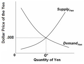
When Americans buy foreign products or make financial investments overseas we demand foreign currency and supply dollars
When foreigners buy American products or make financial investments in the U.S. they demand dollars and supply their currency
DETERMINANTS: Why would Americans demand foreign currency and supply dollars?
To buy more foreign products: PPINT
- Lower prices overseas, higher prices in the US (Pog subs)
- Increase in US incomes (I = Income)
- Increase in tastes for foreign goods (T = tastes)
To invest financially overseas:
- Higher interest rates overseas, lower interest rates in the US
DETERMINANTS: Why would foreigners demand dollars and supply their currency?
To buy more US products: PPINT
- Lower prices in US, higher prices in their country (Pog subs)
- Increase in their incomes (I - Income)
- Increase in tastes for US goods (T=tastes))
To invest financially in the US:
- Higher interest rates in US, lower interest rates in their country
REMEMBER:
- The demand for $ by Mexicans is the same as the supply of pesos. They supply pesos when they buy $.
- The demand for pesos by Americans is the same as the supply of $. We supply $ when we buy pesos.
Graph used to show the effects of a tariff (trade
restriction):
20b Key Graphs
Exchange Rates:
- Episode
35: Why do countries restrict trade?
20b Review Videos
[8:34 YouTube mjmfoodie]
- Foreign
Exchange (FOREX)- Macro 5.2
[8:34 YouTube ACDC Leadership ]
NOTE: These are REVIEW videos only. In order to learn the material you must read the assigned textbook readings, watch the assigned lecture videos, and do problems. See the MACWEBAPP or the LESSONS link for these assignments.
Unit 2: Introduction to
Macroeconomics
Lesson 12a: The AD/AS Model - The AD
Graph and Determinants
In chapter 12 we develop a model of the macroeconomy, the Aggregate
Demand / Aggregate Supply model (AS/AD), that we will use throughout
the remainder of the course. Remember from chapter 1 that the three
macroeconomics issues are unemployment (UE), inflation (IN), and
economic growth (EG). The AD/AS model will help us understand changes
in UE, IN, and EG.
12a Introduction
In lesson 12a we briefly introduce UE, IN, and EG and then develop the aggregate demand curve (AD). In lesson 12b we will develop the aggregate supply (AS) curve and then put them together to find a macroeconomic equilibrium. Then, similar to what we did in chapter 3, we will see that changes in the determinants of AD or AS cause the curves to shift resulting in changes in UE, IN, and EG. LEARN THE DETERMINANTS! See the Yellow Pages for lists of the determinants and many practice exercises.
One last thing, even though the AS/AD graph looks very similar to the supply and demand graph from chapter 3, THEY ARE VERY DIFFERENT. Whereas in chapter 3 we looked at the price and quantity of a SINGLE PRODUCT, in macroeconomics we look at the price level and the aggregate output in the WHOLE ECONOMY. We are not just looking at one product, we are looking at the average prices of ALL products and the quantities of ALL products produced in an economy.
Read the first 5 paragraphs and and paragraph 10 in the link below
where Joseph Stiglitz explains how the lack of Aggregate Demand (AD)
can cause slow or no economic growth around the world.
12a Something Interesting - Why are
we studying this?
Why
the Great Malaise of the World Economy Continues in
2016,
Joseph E. Stiglitz
http://www.huffingtonpost.com/joseph-e-stiglitz/world-economy-2016_b_8908560.html
From Wikipedia: "Joseph Eugene Stiglitz . . . is an American economist and a professor at Columbia University. He is a recipient of the Nobel Memorial Prize in Economic Sciences . . . . He is a former senior vice president and chief economist of the World Bank and is a former member and chairman of the Council of Economic Advisers, [under president Clinton]. . . . Based on academic citations, Stiglitz is the 4th most influential economist in the world today, and in 2011 he was named by Time magazine as one of the 100 most influential people in the world."
12a Assignments: Readings
Ch. 6, pp. 135-140, (19th, 116-120), "Performance and Policy", "The Miracle of Modern Economic Growth",
Ch. 9, pp. (19th, 171-173) "The Business Cycle"
Ch.12, pp. 263-268, (19th, 233-238), "Aggregate Demand", "Changes in Aggregate Demand"
BUSINESS CYCLES
12a Assignments: Video
Lectures
11.1.1 The Business Cycle Recessions, Depressions, and Booms 2:59 [MyNotes]11.1.2 Theoretical Explanations for Cycles 10:09 [MyNotes]
AGGREGATE DEMAND
14.1.1 Deriving the Aggregate Demand Curve 7:26 [MyNotes]14.1.2 Movement along the Aggregate Demand Curve 9:15 [MyNotes]
14.1.3 Shifts in Aggregate Demand 6:03 [MyNotes]
TOPICS
12a Outcomes - What you should
learn
- UE, IN, and EG (Ch 6)
- The business cycle: short-run changes in UE and IN and long-run EG (Ch. 9)
- A model of the macro-economy: AD and its determinants (Ch. 12)
OUTCOMES
- What is the "miracle of modern economic growth"?
- Economic growth, the choice between present and future consumption, and the role of saving and investment.
- Unemployment, inflation and the business cycle: peak, recession, trough, and expansion (recovery); long run growth trend
- Causes of the business cycle: demand shocks and price stickiness
- Define, draw, and describe the shape, and
understand the determinants of the AD curve
[Define, Draw, Describe, Determinants] - How does the AS/AD model of chapter 12 differ from the S/D model of chapter 3?
12a Determinants of AD and AS |
![]() AD__________
AD__________
![]() AD___________
AD___________
![]() C
C ![]()
![]() AD
AD
![]() C
C ![]()
![]() AD
AD
![]() I
I ![]()
![]() AD
AD
![]() I
I ![]()
![]() AD
AD
![]() G
G ![]()
![]() AD
AD
![]() G
G ![]()
![]() AD
AD
![]() Xn
Xn ![]()
![]() AD
AD
![]() Xn
Xn ![]()
![]() AD
AD
![]() MS
MS ![]()
![]() Int. Rt.
Int. Rt. ![]()
![]() I
I ![]()
![]() AD
AD
![]() MS
MS ![]()
![]() Int. Rt.
Int. Rt. ![]()
![]() I
I ![]()
![]() AD
AD
![]() T
T ![]()
![]() C
C ![]()
![]() AD
AD
![]() T
T ![]()
![]() C
C ![]()
![]() AD
AD
![]() S
S ![]()
![]() C
C ![]()
![]() AD
AD
![]() S
S ![]()
![]() C
C ![]()
![]() AD
AD
DETERMINANTS of AD
Consumption (C)
Investment (I)
Government Purchases (G)
Net Exports (Xn)
Money Supply (MS)
Taxes (T)
Saving (S)
DETERMINANTS of AD
C = consumer spending (and saving)
1. consumer wealth
2. consumer expectations
3. consumer indebtedness
4. taxes
I = investment spending
1. interest rates (money supply)
2. profit expectations on investment projects
3. business taxes
4. technology
technology improves5. degree of excess capacity
G = government purchases (no determinants)
Xn = net export spending
1. net income abroad
2. exchange rates
DETERMINANTS of AS
![]() AS__________
AS__________
![]() AS__________
AS__________
![]() price of resources
price of resources ![]()
![]() AS
AS
![]() price of resources
price of resources ![]()
![]() AS
AS
![]() productivity
productivity ![]()
![]() AS
AS
![]() productivity
productivity ![]()
![]() AS
AS
![]() business taxes and gov't red tape
business taxes and gov't red tape ![]()
![]() AS
AS
![]() business taxes and gov't red tape
business taxes and gov't red tape ![]()
![]() AS
AS
DETERMINANTS of AS
Price of Resources
Productivity of Resources
Business Taxes and Gov't Regulations
Key
Terms Flash Cards - Click Here
12a Key Terms
Key Terms:
real GDP, unemployment, inflation, modern economic growth, saving, economic investment, financial investment, business cycle, peak, recession, trough, expansion (recovery), growth trend (secular trend), aggregate demand (AD), real-balances effect, interest-rate effect, foreign-purchases effect, determinants of aggregate demand, wealth vs. income, investment (investment spending)
12a Key Formulas
GDP = C + Ig + G + Xn
The 5Es and Macroeconomic Issues
12a Key Graphs
The Business Cycle
Aggregate Demand (AD)
Increase in AD / Decrease in AD
- Macro
2.7- Business Cycle Unit Summary
12a Review Videos
[1:32 YouTube ACDC Leadership]
- Macro
3.1- Aggregate Demand Practice
[3:21 YouTube ACDC Leadership]
NOTE: These are REVIEW videos only. In order to learn the material you must read the assigned textbook readings, watch the assigned lecture videos, and do problems. See the MACWEBAPP or the LESSONS link for these assignments.
Unit 2: Introduction to
Macroeconomics
Lesson 12b: The AD/AS Model - AS and
Equilibrium in the Macro-Economy
(UE, IN, EG)
(UE, IN, EG)
Almost everyday we can find news about unemployment (UE), inflation
(IN), and economic growth (EG). People discuss these issues over
coffee and presidential candidates discuss them during debates. Our
elected leaders consider them in pieces of legislation. How can we
gain a better understanding of the causes of unemployment, inflation,
and economic growth so that we can better understand these
discussions? To economists the answer is the Aggregate Demand /
Aggregate Supply model of the macroeconomy.
12b Introduction
In this lesson we will add aggregate supply to our aggregate demand graph (lesson 12a) and use the combined graphs to find the equilibrium level of real GDP (output) and price level. We will see what causes the equilibrium level of real GDP (output) and price level of an economy to change (the determinants of AD and AS), and we will use such changes to gain a better understanding of the causes of UE, IN, and EG.
So the next time you hear a politician discuss what they plan to do about UE, IN, and EG, you will have a much better understanding of what the are saying.
Low oil prices boost economic growth:
12b Something Interesting - Why are
we studying this?
"Sinking prices have implications for economies across the globe. Important oil exporters, such as the OPEC countries, bear the brunt of negative impacts, while oil importers benefit. Overall economic activity in the U.S. will benefit, although lower oil prices will depress activity in many producing states, such as Texas and North Dakota..... Depending on which economic model is used, a 50 percent oil price decline yields a 0.3 to 1 percent increase in U.S. GDP. The traditional rule of thumb has been that a sustained 50 percent lower crude oil price raises the growth rate by about 1 percentage point. However, since the U.S. produces more oil and uses it more efficiently nowadays, the traditional rule of thumb should probably be halved—the reduction should boost U.S. growth 0.5 percentage point for a year or so."From: Dallas Fed Vol. 10 No. 3, April 2015, "Economic Letter - Plunging Oil Prices: A Boost for the U.S. Economy, a Jolt for Texas" by Anthony Murphy, Michael Plante and Mine Yücel
https://www.dallasfed.org/assets/documents/research/eclett/2015/el1503.pdf
After this lesson you should be able to use an AS/AD graph to illustrate the effects of low oil prices on the US economy and use the graph to explan what should happen to UE, IN, and EG.
12b Assignments: Readings
Ch. 12, pp. 268- 281, (19th, 238-250), "Aggregate Supply", "Changes in Aggregagte Supply", "Equilibrium in the AD-AS Model", "Changes in Equilibrium"
Ch. 9, pp. 205-206, (19th, 179-180), "Types of Inflation"
Review Ch. 1, pp. 17-19, (19th, 16-18), "Present Choices, Future Possibilities"
AGGREGATE SUPPLY
12b Assignments: Video
Lectures
14.2.1 The Short-Run Aggregate Supply Curve 9:03 [MyNotes]14.2.2 The Labor Market 7:20 [MyNotes]
EQUILIBRIUM
14.3.2 Equilibrium in the Short Run 12:10 [MyNotes]14.3.7 Hot Topic: Oil Shocks 4:52 [MyNotes]
TOPICS
12b Outcomes - What you should
learn
- Aggregate Supply (AS) and its Determinants
- Macroeconomic Equilibrium
- Changes in AD and what happens to UE, IN, and EG
- Changes in AS and what happens to UE, IN, and EG
- Changes in both AD and AS and what happens to UE, IN, and EG
OUTCOMES
- Define, draw, and describe the shape of the
immediate short-run, short-run, and long-run AS curves, and
understand the determinants of the short-run AS curve
[Define, Draw, Describe, Determinants] - Find an economy's equilibrium price level and real domestic output using AD/AS graph
- Explain using an AD/AS graph what happens to RDO, the price level, UE, IN, and EG when there is a change in AD and/or AS.
- Explain the ratchet effect and demand pull inflation
- Explain cost-push inflation and stagflation
- Two (or three) definitions of economic growth
- IN THE NEWS - Use the AS/AD model to
explain what might happen to UE, IN, and EG following these events
in the news:
- 2003: "the recently-signed tax-cut plan, which will give rebate checks to families with children in late summer, right in time for back-to-school spending"
- 2003: "improving consumer confidence -- critical, since consumer spending makes up more than two-thirds of the economy"
- 2003: "The Commerce Department's report last week of a surprising August improvement in the international trade balance "
- 2009: "Personal spending jumped 1.3% last month, the government said."
- 2011: "With energy prices already well on the rise before the latest crisis hit the Middle East and North Africa, is the global economy headed for another tumble?"
- How can an economy go beyond the full employment level of output?
12b Determinants of AD and AS |
![]() AD__________
AD__________
![]() AD___________
AD___________
![]() C
C ![]()
![]() AD
AD
![]() C
C ![]()
![]() AD
AD
![]() I
I ![]()
![]() AD
AD
![]() I
I ![]()
![]() AD
AD
![]() G
G ![]()
![]() AD
AD
![]() G
G ![]()
![]() AD
AD
![]() Xn
Xn ![]()
![]() AD
AD
![]() Xn
Xn ![]()
![]() AD
AD
![]() MS
MS ![]()
![]() Int. Rt.
Int. Rt. ![]()
![]() I
I ![]()
![]() AD
AD
![]() MS
MS ![]()
![]() Int. Rt.
Int. Rt. ![]()
![]() I
I ![]()
![]() AD
AD
![]() T
T ![]()
![]() C
C ![]()
![]() AD
AD
![]() T
T ![]()
![]() C
C ![]()
![]() AD
AD
![]() S
S ![]()
![]() C
C ![]()
![]() AD
AD
![]() S
S ![]()
![]() C
C ![]()
![]() AD
AD
DETERMNANTS of AD
Consumption (C)
Investment (I)
Government Purchases (G)
Net Exports (Xn)
Money Supply (MS)
Taxes (T)
Saving (S)
DETERMINANTS of AD
C = consumer spending (and saving)
1. consumer wealth
2. consumer expectations
3. consumer indebtedness
4. taxes
I = investment spending
1. interest rates (money supply)
2. profit expectations on investment projects
3. business taxes
4. technology
technology improves5. degree of excess capacity
G = government purchases (no determinants)
Xn = net export spending
1. net income abroad
2. exchange rates
Determinants of AS
![]() AS__________
AS__________
![]() AS__________
AS__________
![]() price of resources
price of resources ![]()
![]() AS
AS
![]() price of resources
price of resources ![]()
![]() AS
AS
![]() productivity
productivity ![]()
![]() AS
AS
![]() productivity
productivity ![]()
![]() AS
AS
![]() business taxes and gov't red tape
business taxes and gov't red tape ![]()
![]() AS
AS
![]() business taxes and gov't red tape
business taxes and gov't red tape ![]()
![]() AS
AS
DETERMINANTS OF AS
Price of Resources
Productivity of Resources
Business Taxes and Gov't Regulations
Key
Terms Flash Cards - Click Here
12b Key Terms
Key Terms:
AS, immediate-short-run AS, short-run AS, long-run AS, Keynesian range, Intermediate range, Classical range, equilibrium price level, equilibrium real output (RDO), demand-pull inflation, cost-push inflation, efficiency wages, ratchet effect, stagflation, OPEC
12b Key Problems
Article 2 - The US Economy has Reached a Turning Point
Article 3 - Economy is Bad, but 1982 was worse
Article 4 - Early 1980s Recession
Article 5 - The Roosevelt Recession
Read the following very short news articles, then for each article:
1. Find and CIRCLE the determinants of Aggregate Demand (AD) and/or Aggregate Supply (AS) that have changed.
2. Show the effects of these changes on an AS/AD graph.
3. Show the effects on the equilibrium Price Level (PL) and Real Domestic Output (RDO).
4. State what happens to UE, IN, and EG.
Red Flag: U.S. economy may have hit the pause button, by Patrick Gillespie, April 6, 2016
http://money.cnn.com/2016/04/06/news/economy/us-economy-growth-forecast-first-quarter/index.html?category=economy
Economists have dramatically cut their forecasts for U.S. economic growth in the first quarter of 2016. Falling car sales, equipment purchases by businesses and a downward revision to consumer spending have darkened the view.
The US Economy Has Reached A Turning Point, The Economist, Oct. 5, 2014
http://www.businessinsider.com/the-us-economy-has-reached-a-turning-point-2014-10
The economy powered ahead. . . . [G]rowth was boosted by improvements across all sectors, including consumer spending, residential and non-residential fixed investment, net exports and government spending. . . . Lower energy prices will also provide a lift, reducing business costs. . . .
The Economy Is Bad, but 1982 Was Worse, By DAVID LEONHARDT, JAN. 20, 2009
http://www.nytimes.com/2009/01/21/business/economy/21leonhardt.html
So suffice it to say that the serious recent declines in retail sales, business spending and employment make it highly unusual that the economy will improve anytime soon. . . . [I]t is hard to judge the staggering stimulus numbers being thrown around Washington whether [the Obama administration is] running the risk of being too timid or too aggressive.
1980-82 Early 1980s Recession
http://vm136.lib.berkeley.edu/BANC/ROHO/projects/debt/1980srecession.html
Between 1980 and 1982 the U.S. economy experienced a deep recession, the primary cause of which was the disinflationary monetary policy adopted by the Federal Reserve. The recession coincided with U.S. President Ronald Reagan's steep cuts in domestic spending. [Another] cause of the early 1980s recession was the Iranian Revolution of 1979, which sparked a second large round of oil price increases.
The Roosevelt Recession: (May 1937 - June 1938).
A Review Of Past Recessions By Dan Barufaldi
http://www.investopedia.com/articles/economics/08/past-recessions.asp
Reasons and Causes: The stock market crashed in late 1937.
The Post-Korean War Recession: (July 1953 - May 1954)
A Review Of Past Recessions By Dan Barufaldi
http://www.investopedia.com/articles/economics/08/past-recessions.asp
Reasons and causes: After an inflationary period that followed the Korean War, more dollars were directed at national security. The Federal Reserve tightened monetary policy to curb inflation in 1952.
GDP = C + Ig + G + Xn
12b Key Formulas
Aggregate (AS) Supply
12b Key Graphs
Increase in AS / Decrease in AS
Macroeconomic Equilibrium
Change (Increase) in AD
Change (Increase) in AS
12b Review
Quiz - Lessons 12a and 12b
- Macro
3.2- Aggregate Supply Practice
12b Review Videos
[2:10 YouTube ACDC Leadership]
- Macro
3.3- Long Run Aggregate Supply, Recession, and Inflation
(LRAS)
[Beginning to 1:50 YouTube ACDC Leadership]
NOTE: These are REVIEW videos only. In order to learn the material you must read the assigned textbook readings, watch the assigned lecture videos, and do problems. See the MACWEBAPP or the LESSONS link for these assignments.
Unit 2: Introduction to
Macroeconomics
Lesson 12c: Stabilization Policies and
AS/AD in the Long Run
Now that we have a tool to use to better understand what causes
changes in UE, IN, and EG, let's look at what the government can do
to reduce high UE and high IN. What are the government POLICIES that
can reduce UE and reduce IN?
12c Introduction
Luckily, this is one concept where the terminology used by economists is also used by everybody else. So when you read about "fiscal policy" and "monetary policy" in your textbook and in the newspaper, they mean the same thing!
We will finish this lesson with a review of the economic history of United States. You have all heard about the "Great Depression" (1929-1939). Let's see if we can use what we have learned (the AD/AS model) to better understand its causes and why it ended.
Between December 2007 and June 2009 output in the United States
declined during what became known as "The Great Recession" . This was
followed by a very slow, multi-year, recovery. Economists disagreed
on what should have been done to quicken the recovery:
12c Something Interesting - Why are
we studying this?
ON THE ONE HAND: "The basic issue, says Krugman, is a lack of demand. American consumers and businesses, aren't spending enough, and efforts to get them to open their wallets have gone nowhere. Krugman's solution: The federal government needs to step in and spend. A lot."
May 2, 2012 http://www.rollingstone.com/politics/news/paul-krugman-on-how-to-fix-the-economy-and-why-its-easier-than-you-think-20120502ON THE OTHER HAND: "Is government’s role to fix economy? NO! Just get out of the way and it will fix itself" (The Investment Watchdog Blog).
Sept. 12, 2011 http://investmentwatchblog.com/analysis-is-governments-role-to-fix-economy-no-just-get-out-of-the-way-and-it-will-fix-itself/
President Harry S Truman once said: "I want a one-armed economist, that way he cannot say, 'on the other hand'.
12c Assignments: Readings
Ch. 13, pp. (288-293, (19th, 258-261), "Fiscal Policy and the AD-AS Model"
Ch. 18, pp. 416-420, (19th, 374-378), "Taxation and Aggregate Supply" (Supply-Side Economics)
Ch. 18, pp. 404-410, (19th, 362-368), "From Short Run to Long Run", "Applying the Extended AS-AS Model"
Ch. 18, pp. 411-416, (19th, 368-374, " The Inflation-Unemployment Relationship" (The Phillips Curve)
Summary of Macroeconomic Policy
Fiscal Policy and Economic History of the U.S.
12c Assignments: Video
Lectures
Historical circumstances explained by AD/AS: Demand-pull inflation under Johnson (Khan Academy 9:18)Historical circumstances explained by AD/AS: Real GDP driving price (Khan Academy 6:15)
Historical circumstances explained by AD/AS : Cost-push inflation (Khan Academy 5:45)
Long-Run AS
14.2.3 The Long-Run Aggregate Supply Curve 11:17 [MyNotes]14.3.3 Equilibrium in the Long Run 7:32
14.3.4 Expectations in the Long Run and the Short Run 14:36 [MyNotes]
14.3.5 Long-Run Macroeconomic Equilibrium 16:55 [MyNotes]
Phillips Curve
14.4.1 The Phillips Curve: Definitions and the Historical Record 13:38 [MyNotes]14.4.2 Expectations and the Phillips Curve 9:15 [MyNotes]
TOPICS
12c Outcomes - What you should
learn
- Stabilization Policies
- Fiscal Policy
- Monetary Policy
- Supply-side policy
- AS/AD in the Long Run
- More Practice with the AS/AD Model: Economic history of the U.S.
- The Phillips Curve
OUTCOMES
- Differentiate between expansionary and contractionary fiscal policy and recognize the conditions on an AD/AS graph for recommending an expansionary or contractionary policy.
- Differentiate between easy (expansionary) and tight (contractionary) monetary policy and recognize the conditions on an AD/AS graph for recommending an expansionary or contractionary policy.
- Know how a change in the money supply is
transmitted to a change in AD
[ MS
interest
rates
I
AD]
MS
interest
rates
I
AD] - Supply-side policies and equilibrium output
- Explain long run adjustments to changes in AD and why the long-run aggregate supply curve is a vertical line (LRAS).
- The first paragraph of chapter 18
says:
- "During the early years of the Great
Depression, many economists suggested that the economy would
correct itself in the long run without government intervention.
To this line of thinking, economist John Maynard Keynes
remarked, “In the long run we are all dead!”
Using the AS/AD model explain and show how an econmy will "correct itself" if it has high unemployment.
Using the AS/AD model explain and show how an economy will "correct itself" if it has high inflation.
- "During the early years of the Great
Depression, many economists suggested that the economy would
correct itself in the long run without government intervention.
To this line of thinking, economist John Maynard Keynes
remarked, “In the long run we are all dead!”
- Use the AD/AS model (graph) to explain the economic history of the United States in the past hundred years including the "Great Depression" of 1929-1939 and the "Great Recession" of 2007-2009.
- The Phillips Curve
12c Determinants of AD and AS |
![]() AD__________
AD__________
![]() AD___________
AD___________
![]() C
C ![]()
![]() AD
AD
![]() C
C ![]()
![]() AD
AD
![]() I
I ![]()
![]() AD
AD
![]() I
I ![]()
![]() AD
AD
![]() G
G ![]()
![]() AD
AD
![]() G
G ![]()
![]() AD
AD
![]() Xn
Xn ![]()
![]() AD
AD
![]() Xn
Xn ![]()
![]() AD
AD
![]() MS
MS ![]()
![]() Int. Rt.
Int. Rt. ![]()
![]() I
I ![]()
![]() AD
AD
![]() MS
MS ![]()
![]() Int. Rt.
Int. Rt. ![]()
![]() I
I ![]()
![]() AD
AD
![]() T
T ![]()
![]() C
C ![]()
![]() AD
AD
![]() T
T ![]()
![]() C
C ![]()
![]() AD
AD
![]() S
S ![]()
![]() C
C ![]()
![]() AD
AD
![]() S
S ![]()
![]() C
C ![]()
![]() AD
AD
DETERMNANTS of AD
Consumption (C)
Investment (I)
Government Purchases (G)
Net Exports (Xn)
Money Supply (MS)
Taxes (T)
Saving (S)
DETERMINANTS of AD
C = consumer spending (and saving)
1. consumer wealth
2. consumer expectations
3. consumer indebtedness
4. taxes
I = investment spending
1. interest rates (money supply)
2. profit expectations on investment projects
3. business taxes
4. technology
technology improves5. degree of excess capacity
G = government purchases (no determinants)
Xn = net export spending
1. net income abroad
2. exchange rates
Determinants of AS
![]() AS__________
AS__________
![]() AS__________
AS__________
![]() price of resources
price of resources ![]()
![]() AS
AS
![]() price of resources
price of resources ![]()
![]() AS
AS
![]() productivity
productivity ![]()
![]() AS
AS
![]() productivity
productivity ![]()
![]() AS
AS
![]() business taxes and gov't red tape
business taxes and gov't red tape ![]()
![]() AS
AS
![]() business taxes and gov't red tape
business taxes and gov't red tape ![]()
![]() AS
AS
DETERMINANTS OF AS
Price of Resources
Productivity of Resources
Business Taxes and Gov't Regulations
Key
Terms Flash Cards - Click Here
12c Key Terms
Key Terms:
stabilization policies, demand management, fiscal policy (FP), expansionary FP, contractionary FP, monetary policy (MP), easy (expansionary) MP, tight (contractionary) MP, supply-side policy, Laffer curve, stagflation, aggregate supply shocks, short run, long run, long-run AS, Phillips curve, long-run Phillips Curve, the Great Depression, disinflation
12c Macroeconomic
Policies
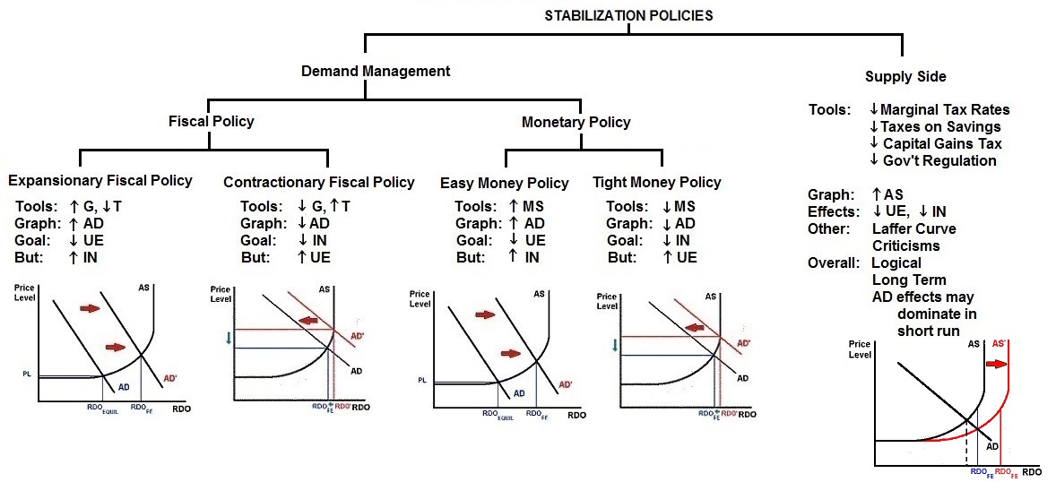
Laffer Curve
12c Key Graphs
Long Run AS
Long Run AS - Adjusting to an increase in AD
Long Run AS - Adjusting to a decrease in AD
Philips Curve
- Fiscal
& Monetary Policy Review- AP
Macroeconomics 3:58
12c Review Videos
[YouTube ACDC Leadership]
- Macro
3.3- Long Run Aggregate Supply, Recession, and Inflation
(LRAS)
[1:50 to end YouTube ACDC Leadership]
- The
Phillips Curve (Macro Review) Macro 3.4
[3:15 to end YouTube ACDC Leadership]
NOTE: These are REVIEW videos only. In order to learn the material you must read the assigned textbook readings, watch the assigned lecture videos, and do problems. See the MACWEBAPP or the LESSONS link for these assignments.
Unit 2: Introduction to
Macroeconomics
Lesson 9a: Unemployment
(UE)
Most economists will say that the U.S. economy achieves full
employment at an UE rate of about 5%. Five percent unemployment in
the U.S. is about eight million people unemployed and THAT is called
full employment. How can 8 million unemployed people be called "full
employment"? How is the unemployment rate calculated? Who is
employed? Who is unemployed? What is "full" employment? What is
"unemployment"?
9a Introduction
We will try to understand the answers to these questions by returning to the 5Es of economics from lesson 1b. We learned there that the 5 Es were five ways to reduce scarcity and achieve the maximum level of satisfaction for a society. In the U.S. we can produce the maximum amount of output when there is about 5% unemployment. Confusing? Yes. It should be - - - now, but after studing this lesson it will be much more clear.
205,000 jobs created in March, 2016, but the unemployment rate
increases. WHY?.
9a Something Interesting - Why are we
studying this?
"The American economy continues its march upward. The monthly jobs report released Friday by the Bureau of Labor Statistics showed that the economy created 215,000 jobs in March, slightly higher than the 205,000 expected. The unemployment rate ticked up to 5 percent from 4.9 percent. U.S. job growth has continued for a record 73 months in a row."The Huffington Post 04/01/2016 09:58 am ET.
How can there be both more jobs and more unemployment ?
This news article linked below also says: "the increase in the unemployment rate is actually a good thing". How can that be?
Read the first five paragraphs of the article linked below to find out.
http://www.huffingtonpost.com/entry/march-jobs-report_us_56fe6c5de4b0a06d58056916
Most economists will say that when the U.S. economy achieves an UE rate of about 4 to 5%, then we have achieved full employment. Four to Five percent unemployment in the U.S. is about six and a half to eight million people unemployed and THAT is full employment. How can that be?
Who is counted when they calculate the unemployment rate? And who is not counted?
Watch the short YouTube video linked below.
The Unemployment Game Show: Are You *Really* Unemployed? from Mint.com 2:10
9a Assignments: Readings
Ch. 9, pp. 198-204, (19th, 173-179), "Unemployment"
Unemployment Rate in the United States
11.2.1 Measuring
the Labor Force and Unemployment 5:48
[MyNotes]
9a Assignments: Video
Lectures
The Unemployment Game Show: Are You *Really* Unemployed? from Mint.com 2:10
11.2.2 Types of Unemployment 4:18 [MyNotes]
11.3.1 Understanding the Natural Rate of Unemployment 4:05 [MyNotes]
TOPICS
9a Outcomes - What you should
learn
- What is Unemployment?
- Who is included and who is not?
- The Unemployment Rate and the "Real" Rate of Unemployment
- What is Full Employment and the Types of
Unemployment?
- The Natural Rate of Unemployment
- Changes in the Natural Rate of Unemployment
- The Costs of Unemployment
OUTCOMES
- What is unemployment? Describe how unemployment is measured. How is the unemployment rate calculated? Who is included as employed, unemployed, and who is not in the labor force?
- Why might UE increase as an economy is beginning to recover from a recession?
- Define the "Real Rate of UE".
- What is full employment? Identify the full employment, or natural rate, of unemployment and explain why 5% unemploymnent can be called full employment.
- Define and give examples of frictional, cyclical, and structural unemployment.
- How and why has the natural rate of unemployment changed over the past five or six decades?
- Why might UE increase as an economy is beginning to recover?
- Jan. 2015: US population 320,090,000; US
labor force 157,180,000
Sept. 2015: US population 321,650,000; US labor force 156,715,000
How can the size of the labor force decline as the size of the population increases? - Identify the economic costs of unemployment and the groups that bear unusually heavy unemployment burdens.
- What is a positive GDP gap and a negative GDP gap?
Key
Terms Flash Cards - Click Here
9a Key Terms
Key Terms:
unemployment rate, unemployed, employed, labor force, underemployed, discouraged worker, "natural rate of UE" or "full employment rate of UE", "real rate of UE", frictional UE, structural UE, cyclical UE, potential output, GDP gap, labor force participation rate
9a Key Formulas
9a Key Formulas
Unemployment Rate = (# UE / # labor force) x 100
9a Key Graphs
Point D represents unemployment (or productive inefficiency)
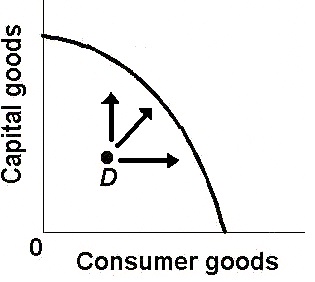
AS/AD Graph representing an economy with unemployment
- Macro
2.3- Unemployment and Natural Rate of Unemployment- AP
Macro
9a Review Videos
[1:54 YouTube ACDC Leadership]
- Unemployment
Game Show - Are you Officially Unemployed?
[2:09 YouTube Mint.com]
NOTE: These are REVIEW videos only. In order to learn the material you must read the assigned textbook readings, watch the assigned lecture videos, and do problems. See the MACWEBAPP or the LESSONS link for these assignments.
Unit 2: Introduction to
Macroeconomics
Lesson 9b: Inflation
(IN)
The THREE ISSUES of Macroeconomics are: UE, IN, and EG. In chapter
12 we learned a tool (the AS/AD model) that helped us understand what
causes UE, IN, and EG. Chapter 9 discusses the issues of UE and IN in
greater detail. And in chapters 7, 8 and 22W we study EG.
9b Introduction
We have already learned two causes of inflation (lesson 12b), demand-pull and cost-push inflation, but we really did not define inflation. Inflation (IN) is the rate of increase in the price level, i.e. how fast it is increasing. Here we will learn how the price level is measured by using a price index, how inflation is calculated, and the economic effects of inflation.
9b Something Interesting - Why are we
studying this?
Read "Fact 1 Adjusted for inflation, the federal minimum wage peaked in 1968" in the short 2017 news article below about the effects of inflation on the minimum wage.
http://www.pewresearch.org/fact-tank/2017/01/04/5-facts-about-the-minimum-wage/
After reading the article you should be wondering "What causes inflation and what can be done about it?". After studying this lesson you should have a better answer to that question.
OPTIONAL, but interesting:
- http://www.huffingtonpost.com/2013/02/13/minimum-wage-productivity_n_2680639.html
- http://www.businessinsider.com/heres-how-seniors-have-been-getting-screwed-by-how-we-calculate-social-security-2013-11
9b Assignments: Readings
Ch. 9, pp. 204-213, (19th, 179-187), "Inflation", "Redistribution Effects of Inflation", Does inflatin Affect Output?"
Ch. 12, p. 277 (19th, 247) "disinflation" at the bottom of the first column
Ch. 7, pp. 163-164, (19th, 141-142), "GDP Price Index"
Ch. 14, pp. 319-320, (19th, 285-286), "Money and Prices", "Stabilizing Money's Purchasing Power"
11.5.1 Inflation,
Deflation, Stagflation, and Hyperinflation
4:54 [MyNotes]
9b Assignments: Video
Lectures
10.3.1 Changes in the Cost of Living and the CPI 4:47 [MyNotes]
10.3.2 Calculating the Rate of Inflation 7:33 [MyNotes]
10.3.3 Comparing the CPI and the GDP Deflator 6:02 [MyNotes]
11.5.2 Inflation and Purchasing Power 7:45 [MyNotes]
11.5.3 Short-Run Causes: Demand-Pull and Cost-Push Inflation 9:59 [MyNotes]
11.5.5 The Costs of Inflation 9:23 [MyNotes]
11.5.6 Case Study: Behavior during Hyperinflation 6:14 [MyNotes]
TOPICS
9b Outcomes - What you should
learn
- Definition of Inflation
- What is an Index?
- Calculate the Inflation Rate using an Index
- Causes and Effects of Inflation
- Costs of Inflation
OUTCOMES
- Define inflation, deflation, and disinflation
- Calculate the inflation rate using price index data
- What is a price index and how is the CPI measured?
- Explain the two types of inflation (demand-pull; cost-push) using the AD/AS graph
- What is the rule of 70 and apply it to the price level.
- If the population of a country is 25 million and it is growing a rate of 4% a year, how many years will it take for the population to reach 50 million? 100 million? 200 million (assuming that the growth rate stays at 4%)?
- Who is hurt by unanticipated inflation and who may benefit from unanticipated inflation. (redistributive effects of inflation).
- What are the output and employment effects of demand-pull and cost-push inflation? (Who is hurt and who is helped?)
- How does the inflation rate affect real income growth?
- Recently a teachers' union argued that the standard of living of teachers working for the school district was falling. The negotiating team for the school board replied that this was not true because the teachers had received significant increases in nominal income through collective bargaining. Could the union statement be correct?
- If inflation is going down then what is happening to the average level of prices in an economy. OR what is the difference between deflation and disinflation?
Key
Terms Flash Cards - Click Here
9b Key Terms
Key Terms:
inflation, inflation rate, deflation, disinflation, price index, CPI, purchasing power, rule of 70, cost-push inflation, demand-pull inflation, redistributive effects, output effects, hyperinflation, nominal income, real income, COLAs, menu costs
9b Key Formulas
To measure inflation, subtract last year's price index from this year's price index and divide by last year's index; then multiply by 100 to express as a percentage.
Inflation Rate = [ (Price Index this year -
Price Index last year) / Price Index last year ] x 100
IN rate 2015 = [ (PI 2015 - PI 2014) / PI 2014 ] x
100
Demand-Pull Inflation
9b Key Graphs
Cost-Push Inflation
9b Review
Quiz Lessons 9a and 9b
- UE and IN
- Inflation-
Cost-push & Demand-pull- Macro 3.6
9b Review Videos
[5:35 YouTube ACDC Leadership]
NOTE: These are REVIEW videos only. In order to learn the material you must read the assigned textbook readings, watch the assigned lecture videos, and do problems. See the MACWEBAPP or the LESSONS link for these assignments.
Unit 2: Introduction to
Macroeconomics
Lesson 7a: Measuring the Economy -
GDP
Now we begin a three chapter (7, 8, and 22W) discussion
of economic growth (EG).
7a Introduction
Defining EG can be a little complicated and we will study that in the next chapter, but EG usually means "an increase in real domestic output (RDO)". In chapter 7 we learn how real domestic output (RDO) is measured.
We have been using the AS/AD model for several lessons now but we do not know what numbers actually go on the axes of the graph. What numbers do we use to measure RDO on the horizontal axis of the AS/AD graph.? Well, we use real GDP to measure RDO and here we learn how it is calculated. In lesson 9b we learned how a price index (CPI or GDP Index) measures the price level. We use price index numbers on the vertical axis of the AS/AD graph.
Watch this short four minute video from MRuniversity.com
7a Something Interesting - Why are we
studying this?
Interesting video but there is a MAJOR ERROR. It should be called "Basic Facts of INCOME", not WEALTH. The video discusses differences in annual income measured by GDP per capita. Income is not the same as wealth. Income measures how much is produced, or earned, over a period of time, usually one year. That is what the video is talking about. Wealth measures the net worth of a person, the total value of assets minus liabilities (what is owned minus what is owed). The video demonstrates that income is very unequally distributed, but the distribution of wealth is much more unequal.
But how is GDP (or income) measured? Study this lesson to find out.
7a Assignments: Readings
Ch. 7 - ALL
AGGREGATE OUTPUT AND INCOME
7a Assignments: Video
Lectures
10.1.1 The Production Possibilities Frontier: Macroeconomic Applications 18:18 [MyNotes]REVIEW (2a): 10.1.2 The Circular Flow Model 9:38 [MyNotes]
10.1.3 Real GDP 12:01 [MyNotes]
10.1.4 The BEA Procedure for Calculating Real GDP 8:15 [MyNotes]
10.1.5 Limitations of GDP and Alternative Indexes 4:51 [MyNotes]
APPROACHES TO CALCULATING GDP
10.2.1 The Expenditures Approach 4:54 [MyNotes]10.2.2 The Income Approach 7:02 [MyNotes]
EconMovies- Episode 6: Back to the Future (Nominal vs. Real, Unemployment, Inflation) (6:29)
TOPICS
7a Outcomes - What you should
learn
- Define GDP
- Problems (Shortcomings) with using GDP as a Measure of Social Welfare
- Define and Calculate
- GDP
- National Income (NI)
- NDP
- net investment (In)
- net exports (Xn)
- real GDP
- Define Personal Income and Disposable Income
OUTCOMES
- Use a circular flow diagram to show the two ways of calculating GDP
- Define and calculate GDP and NI when given national income data.
- Define and give examples of final goods, intermediate goods, and double counting.
- Differentiate between gross and net investment.
- Define Investment and state what is included. Explain why changes in inventories are investments.
- Calculate net investment and explain how it indicates a growing, static, or declining economy.
- Explain why imports are subtracted to calculate GDP
- List and explain the shortcomings of using GDP as a measure of social welfare.
- India's GDP is much greater than is Switzerland's GDP yet Switzerland has a higher standard of living. Explain.
- After a major natural disaster (flood, tornado, earthquake) GDP often increases. Is GDP in this case a good indicator of social welfare? Explain.
- Find real GDP by adjusting nominal GDP with use of a price index (GDP price index, also called the GDP deflator) and be able to find the years of recessions given nominal GDP data.
Key
Terms Flash Cards - Click Here
7a Key Terms
Key Terms:
Gross Domestic Product (GDP), intermediate goods, final goods, double counting (multiple counting), non-market transactions, underground economy, GDP per capita, expenditures approach, income approach, national income (NI), proprietor's income, personal income (PI), disposable income (DI), nominal GDP, real GDP, gross private domestic investment, net private domestic investment, net domestic product (NDP), net exports
7a Key Formulas
GDP = C + Ig + G + Xn
NI = wages + rents + interest + corporate profits + proprietor's income
NDP = C + In + G + Xn
NDP = GDP - depreciation
In = Ig - depreciation
Xn = X - M
real GDP = (nominal GDP / price index) x 100
Circular Flow Model
7a Key Graphs
7a Review
Quiz
- Macro
Unit 2.1- GDP and Economic Growth
7a Review Videos
[3:37 YouTube ACDC Leadership]
NOTE: These are REVIEW videos only. In order to learn the material you must read the assigned textbook readings, watch the assigned lecture videos, and do problems. See the MACWEBAPP or the LESSONS link for these assignments.
Unit 2: Introduction to
Macroeconomics
Lesson 8a: Economic Growth
(EG)
In chapter 8 the textbook says that there are TWO DEFINITIONS of EG,
but in chapter 1 (Lessons 1b and 1c) we learned another definition.
So actually there are THREE DEFINITIONS of EG.
8a Introduction
I believe the best way of understanding the difference between them is to discuss whether the growth is ACHIEVING THE POTENTIAL of the economy or INCREASING THE POTENTIAL of the economy. Both of these increase RDO (real domestic output) and it is an increase in RDO that is the COMMON DEFINITION of EG. But this everyday definition of economic growth, the one you hear on the news broadcasts, doesn't tell us if the economy is achieving its potential by producing more OR whether the economy is has increased it potential and therefore is ABLE to produce more.
Why is this distinction important? Why do we care? Well, there are different CAUSES and POLICIES for each approach to growth and both approaches increase output and therefore reduce scarcity and increase society's satisfaction. As we should remember from lesson 1b, reducing scarcity and increasing society's satisfaction is the goal of economics.
The economic growth that we are used to, 1%, 2,% 3%, 4%, maybe even,
7%, 8% or even 9% a year, is a recent phenomonon in the history of
the world. Prior to the beginning of the 17th century, (around 1800)
all parts of the world had similar living standards and these living
standards had not changed much for thousands of years. See graph
below.
8a Something Interesting - Why are we
studying this?
Now we expect long term economic growth and living standards in different parts of the world to vary significantly.
Why? We will study this and other econmic growth issues in this lesson.
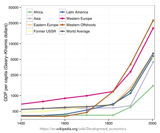
8a Assignments: Readings
Ch. 8 - ALL
Ch. 1, pp. 16-20, (19th, 15-18), "A Growing Economy" and "Present Choices and Future Possibilities"
16.1.2 The
PPF, the AD/AS Model, and Long-Run Growth
7:44 [MyNotes]
8a Assignments: Video
Lectures
16.1.3 The Production Function and Growth 6:49 [MyNotes]
16.1.4 The Definition of Productivity and Factors Affecting It 3:54 [MyNotes]
TOPICS
8a Outcomes - What you should
learn
- Definitions of EG
- EG in the US
- Modern EG
- Determinants of EG
- Causes of Productivity Growth
OUTCOMES
- Give three definitions of economic growth and illustrate them on the 5Es, PPC, AS/AD, and LRAS models.
- Use the 5Es, PPC, AS/AD, and LRAS models to differenciate between "achieving our potential" and "increasing our potential".
- Explain why growth is a desirable goal.
- Define “modern economic growth” , "great divergence", "leading country", and "follower country".
- Identify two main sources of growth (more resources, more productivity) and apply them to the growth history of the United States.
- Explain and apply the "rule of 70."
- Identify and explain the supply factors (INCREASING the potential)
- Identify and explain the demand, and efficiency factors (ACHIEVING the potential)
- Differentiate between ACHIEVING the potential and INCREASING the potential using the PPC. AD/AD, and long-run AS models
- According to the authors, why is the real GDP per capita of the United States in 2007 so much higher than that of other rich countries?
- Differentiate between production, productive efficiency, and productivity
- If the quantity of labor increases, what happens to productivity? ANSWER: Nothing. The quantity of labor will affect production, but the quality of labor affects productivity
- What are the determinants of productivity growth?
- Identify and explain the arguments for and against economic growth.
Key
Terms Flash Cards - Click Here
8a Key Terms
Key Terms:
economic growth, increasing the potential, achieving the potential, GDP per capita, rule of 70, productivity, production, productive efficiency, modern economic growth, the great divergence, leader countries, follower countries, property rights, patents and copyrights, simultaneous consumption, network effects, labor force participation, infrastructure, human capital, economies of scale
GDP per capita = GDP / population
8a Key Formulas
Modern Economic Growth
8a Key Graphs
Economic Growth and the 5Es:
Economic Growth is "Increasing the Potential"
Prod. Eff. and Full Emp[loyment is "Achieving the Potential.
EG - INCREASING THE POTENTIAL
EG - ACHIEVING THE POTENTIAL
EG - ACHIEVING THE POTENTIAL
EG - INCREASING THE POTENTIAL
EG - INCREASING THE POTENTIAL
8a Review
Quiz
- Economic
Growth and LRAS- Macro 3.14
8a Review Videos
[2:58 YouTube ACDC Leadership]
NOTE: These are REVIEW videos only. In order to learn the material you must read the assigned textbook readings, watch the assigned lecture videos, and do problems. See the MACWEBAPP or the LESSONS link for these assignments.
Unit 2: Introduction to
Macroeconomics
Lesson 22Wa: Economic Growth in
the Less Developed Countries (LDCs)
From the United Nations:
22Wa Introduction
- 925 million people do not have enough to eat - more than the combined populations of the USA, Canada, and the European Union; (Source: FAO news release, 14 September 2010)- Nearly half the world’s population, 2.8 billion people, survive on less than $2 a day.
- About 20 percent of the world’s population, 1.2 billion people, live on less than $1 a day.
- Nearly 1 billion people are illiterate and 1 billion do not have safe water.
- 98 percent of the world's hungry live in developing countries; (Source: FAO news release, 2010)
Source:
http://www.un.org/en/globalissues/briefingpapers/food/vitalstats.shtml
I believe that no discussion of EG is complete without a discussion of the world's poor where EG means more than getting a new car or another vacation -- it is a matter of life and death.
A discussion of the world's less developed countries also allows us to return to the subject of STRUCTURAL ADJUSTMENT (globalization) that we studied in unit 1. This would be a good time to review your notes from lesson 2a. Because of the economic growth that has resulted from Structural Adjustment in the past few decades, millions of people in the less developed countries have been lifted out of poverty.
The figure below shows the great decline in the number of people living on $1.25 a day or less since 1990.
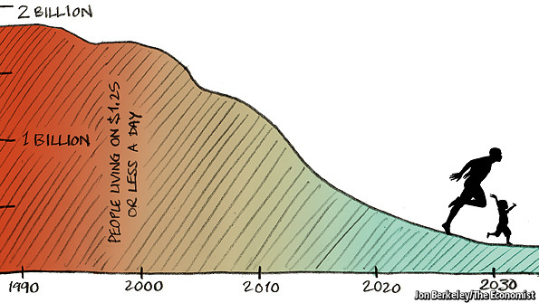
22Wa Something Interesting - Why are
we studying this?
Jan. 2014: "The 85 richest people on Earth now have the same amount of wealth as the bottom half of the global population, according to a report released Monday by the British humanitarian group Oxfam International."
From: Oxfam report highlights widening income gap between rich, poor
Jan. 2018: "Inequality gap widens as 42 people hold same wealth as 3.7bn poorest "
From: https://www.theguardian.com/inequality/2018/jan/22/inequality-gap-widens-as-42-people-hold-same-wealth-as-37bn-poorest
42 people's wealth = 3,700,000,000 people's wealth.
And, the gap between the rich and the poor is widening.
Think about it. In this lesson we will begin to understand why.
22Wa Assignments:
Readings
Ch. 22W - ALL - found online at: Chapter 22W
Also read: Measures of EconomicDevelopment
Oxfam report highlights widening income gap between rich, poor
16.3.1 Growth in
Emerging Economies 10:23
[MyNotes]
22Wa Assignments: Video
Lectures
10.1.6 The Growth of China as a Superpower 2:14 [MyNotes]
16.3.2 Policies to Promote Growth 7:50 [MyNotes]
16.2.2 Other Policies to Encourage Growth 10:40 [MyNotes]
16.3.3 Hot Topic: The Myth of Exploding Populations 8:00 [MyNotes]
16.2.3 Hot Topic: Women's Roles in Rural Economic Growth 4:59 [MyNotes]
TOPICS
22Wa Outcomes - What you should
learn
- The International Distribution of Income
- Characteristics of the LDCS (DVCs)
- Obstacles to Development and the Role of Government
OUTCOMES
- Identify various terms that are used to name the rich and poor countries, including the "global south" and have a general understanding of where thay are on a world map.
- Where do most of the world's people live?
- Why does Africa look so small on many maps?
- Describe the world distribution of wealth
- What is the "vicious cycle" and how does population growth affect it?
- How is the level of saving related to the level of investment and productivity in the cycle of poverty?
- How is the level of saving related to the level of investment and productivity in the cycle of poverty?
- Identify the characteristics of DVCs.
- How does population growth affect the growth in GDP per capita?
- Where did Maltus go wrong?
- Define and give examples of the primary, secondary, and tertiary sectors of an economy
- List some of the obstacles to economic development.
- Discuss the role of the DVC government in promoting economic development within their country
- Describe how IACs can help low-income countries including the trade vs. aid debate
- How can agricultural subsidies in the IACs (MDCs) negatively affect economic growth in the DVCs (LDCs)?
- Describe the growth rates of IACs and DVCs and the growing absolute income gap between rich and poor countries.
Key
Terms Flash Cards - Click Here
22Wa Key Terms
Key Terms:
LDCs (DVCs), MDCs (IACs), global south, primary activities, secondary activities, tertiary activities, vicious circle of poverty, brain drain, land reform, microfinance and Grameen Bank, World Bank, foreign direct investment, GDP per capita, capital flight, supply chain, Malthus, green revolution, financial intermediary
Income per capita: Low, Middle, and High Income Countries
22Wa Key Graphs / Figures
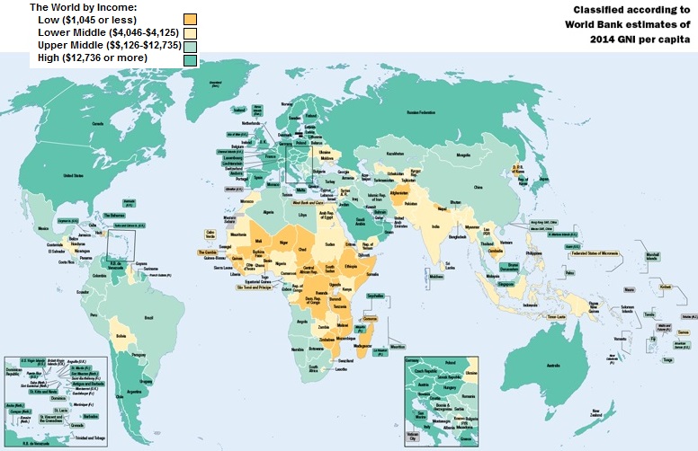
The True Size of the Continents (yellow) and the Size Seen on Many Maps (black outline)
22Wa Review
Quiz
- Economic
Growth in the Less Developed Countries
22Wa Review Videos
[9:45 YouTube Brad Cartwright Economics]
NOTE: These are REVIEW videos only. In order to learn the material you must read the assigned textbook readings, watch the assigned lecture videos, and do problems. See the MACWEBAPP or the LESSONS link for these assignments.
Unit 3: Macroeconomic
Policy
Lesson 14a: Monetary Policy - Money,
The Money Market Model, and the Fed
We now begin unit 3 where we focus on macroeconomic POLICY. When we
say "policy" we mean "government". What can the government do to
achieve the three macroeconomic goals of low UE, low IN, and rapid
EG? In lesson 12c we introduced stabilization policies: monetary
policy and fiscal policy. (This would be a good time to review your
notes on lesson 12c.) Here, we will dig deeper, beginning with
Monetary Policy (MP).
14a Introduction
In lesson 12c we learned that if UE is high we can increase the money supply (MS) which will cause interest rates to go down. We called this an "Easy Money Policy". Lower interest rates will increase investment (I) and therefore increase aggregate demand (AD). When AD increases it will increase real domestic output (RDO or real GDP) and decrease UE. But, it may increase the price level (PL) and therefore increase inflation.
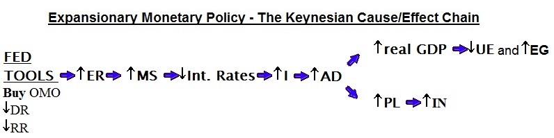
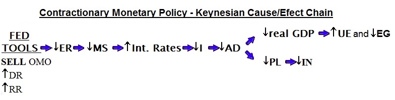
We begin monetary policy in lesson 14a by defining money (what is money?) and the money supply (MS). Then we will develop the model (graphs) of the money market that we will use in the next three chapters to show how monetary policy works. We finish the lesson with a discussion of the structure of the Federal Reserve (the Fed). As we know from lesson 12a the Fed controls the money supply (MS). Here we learn that "the Fed" is NOT the federal government in Washington DC.
The policy making arm of the Fed is basically the Federal Open Market Committee (FOMC) comprised of 12 people and these 12 people have the power to raise interest rates and put millions of people of work as they did in the early 1980s. Or, the FOMC can lower interest rates causing millions of people to earn less on their financial investments. The chairperson of the Fed (Jerome Powell in 2018) has been called "the second most powerful person in the United States". In this unit we will learn why.
Listen or read the link below.
14a Something Interesting - Why are
we studying this?
Planet Money Episode
421: The Birth Of The Dollar Bill
(10:37).
Before the Civil War, there were 8,000 different kinds of money in the United States.Banks printed their own paper money. And, unlike today, a $1 bill wasn't always worth $1. Sometimes people took the bills at face value. Sometimes they accepted them at a discount (a $1 bill might only be worth 90 cents, say). Sometimes people rejected certain bills altogether.
Pictures of early money:
Pre-Civil War Bank Note
So, WHAT IS MONEY? Study this lesson for the answer.
14a Assignments: Readings
Ch. 14, ALL
Ch. 10, pp. 226-231, "The Interest Rate-Investment Relationship" (19th, 199-204)
Ch. 16, pp. 351-354, "Interest Rates", (19th, 315-317)
Ch. 16, pp. 365-367, "Cause-Effect Chain" (19th, 329-330)
Planet Money Episode 421: The Birth Of The Dollar Bill (10:37). Audio only. Interesting radio story on early money in the US.
Pictures of early money:
- Pre-Civil War Bank Note
13.1.1 The
Money Supply 8:10 [MyNotes]
14a Assignments: Video
Lectures
13.4.2 Case Study: Cigarettes As Money 6:07 [MyNotes]
13.1.2 Determinants of Money Demand 9:00 [MyNotes]
13.1.3 The Money Market 10:02 [MyNotes]
Money Market - Macro Review 3:24 [YouTube ACDCLeadership]
13.3.1 The Federal Reserve System 8:13 [MyNotes]
TOPICS
14a Outcomes - What you should
learn
- What is Money?
- The Money Market Model: MD (money demand) and MS (money supply)
- The Structutre and Functions of the Federal Reserve and Banking Systems
OUTCOMES
- Why is money important? Why do we use money? Why do we care about money? What is wrong with barter?
- What is money? How can cigarettes or beer be money?
- List and explain the three functions of money.
- Define the money supply M1, and near monies M2.
- Identify two types of demand for money and the main determinant of each.
- The money market graph: explain what is meant by equilibrium in the money market and the equilibrium rate of interest; what happens when there is a change in the money supply?
- What causes interest rates to change?
- Describe the structure of the U.S. banking system.
- Explain why Federal Reserve Banks are central banks, quasi public banks, and bankers' banks.
- Describe the functions of the Federal Reserve System and point out which role is the most important.
Key
Terms Flash Cards - Click Here
14a Key Terms
Key Terms:
barter, coincidence of wants, money, medium of exchange, unit of account, store of value, commodity money, near money, liquidity, M1, M2, money supply (MS), federal reserve notes, checkable deposits, money demand (total money demand), transactions demand, asset demand, money market model, Federal Reserve System, Board of Governors, FOMC
Money Demand
14a Key Graphs
- D1 is Transactions Demand
- D2 is Asset Demand
Money Market
Increase in the Money Supply
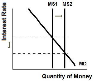
Decrease in the Money Supply
14a Review
Quiz
- Macro
4.2- Functions of Money
14a Review Videos
[2:01 YouTube ACDC Leadership]
- The
Money Market- Macroeconomics 4.6
[3:24 YouTube ACDC Leadership]
- Macro
4.5- The Federal Reserve System- Quick
Overview
[1:59 YouTube ACDC Leadership]
NOTE: These are REVIEW videos only. In order to learn the material you must read the assigned textbook readings, watch the assigned lecture videos, and do problems. See the MACWEBAPP or the LESSONS link for these assignments.
Unit 3: Macroeconomic
Policy
Lesson 15a: Monetary Policy - How
Banks Create Money
Most students are very surprised when they learn that when banks
make loans they create money. Yes, banks create money whenever they
make a loan. If I get a loan from a bank to buy a new boat, the money
I get has been CREATED by the bank. The US government does not create
money. The Federal Reserve does not create money. BANKS CREATE MONEY.
BUT, the Fed can control how much money banks can create. We will
learn how the Fed does this in the next lesson (16a). Here we learn
HOW BANKS CREATE MONEY.
15a Introduction
Watch this short clip from the Christmas movie It's a Wonderful
Life:
15a Something Interesting - Why are
we studying this?
It's
a Wonderful Life Bank Run
Then read the first two short sections on the
webpage linked below: "Definition of a Bank Run" and "How Banks Work:
Demand Deposits" (only 8 short paragraphs). You may have to tap
"Show Full Article" to see "How Banks Work: Demand
Deposits"
What
is a Bank Run?
After studying this lesson you should understand how bank runs may occur.
15a Assignments: Readings
Ch. 15, ALL
13.4.1 How
Goldsmiths Created Money 7:40
[MyNotes]
15a Assignments: Video
Lectures
How banks create money and the money multiplier 4:12 [YouTube ACDCLeadership]
13.4.3 How Banks Create Money 12:09 [MyNotes]
TOPICS
15a Outcomes - What you should
learn
- Goldsmith Banking: the origin of the fractional reserve system of banking
- How Banks Create Money
- The Money Multiplier
OUTCOMES
- Recount the story of how fractional reserves began with goldsmiths.
- Explain a "run on a bank" and how it is related to fractional reserve banking?
- Do banks really "create" money?
- Explain the effects of a currency deposit ($10 bill) in a checking account on the composition and size of the money supply.
- Compute a bank's required and excess reserves when you are given its balance sheet figures.
- Explain why a commercial bank is required to maintain a reserve (required reserve) and why it isn't enough to cover deposits.
- Describe what happens to the money supply when a commercial bank makes a loan or buys securities. Describe what happens to the money supply when a loan is repaid or a bank sells its securities.
- Explain what happens to a commercial bank's reserves and checkable deposits after it has made a loan.
- Describe how a check drawn on one commercial bank and deposited in another will affect the reserves and excess reserves in each bank after the check clears.
- Explain how it is possible for the banking system to create an amount of money that is a multiple of its excess reserves when no single bank ever creates money greater than its excess reserves.
- Compute the size of the monetary multiplier and the money creating potential of the banking system when provided with appropriate data.
Key
Terms Flash Cards - Click Here
15a Key Terms
Key Terms:
fractional reserve banking system, goldsmith banking, balance sheet (T-account), assets, liabilities, assets of a commercial bank, liabilities of a commercial bank, reserves (total reserves or actual reserves), reserve ratio, required reserves, excess reserves (lendable reserves), demand deposit, check clearing, money multiplier (deposit expansion multiplier, monetary multiplier), government securities or bonds, net worth (owner's equity), run on a bank (bank run)
Money
Creation - Single Bank and Banking System
15a Key Problems
ASSETS LIABILITIES + NET WORTH
Reserves $ 200 Checkable Deposits $ 600
Loans 100 Stock Shares 700
Securities 500
Property 500
Refer to the above information for a single bank. The required (legal) reserve ratio is 25%. This bank can safely expand its loans by a maximum of:
1. $0
2. $50
3. $100
4. $200
Refer to the above information. The required (legal) reserve ratio is 25%. If the original bank balance sheet was for the commercial banking system, rather than a single bank, loans and deposits could have been expanded by a maximum of:
1. $0
2. $50
3. $100
4. $200
What is your answer to the question above if the Fed lowered the Required Reserve ratio to 20%?
1. $200
2. $250
3. $400
4. $600
Money Creation Problem - Single Bank and Banking System
15a Key Formulas
Total Change in Money Supply = Initial excess reserves x Money Multiplier
Total Reserves = Cash in vault + Deposits at Fed
Required Reserves = Reserve Requirement x Liabilities
Excess Reserves = Total Reserves - Required Reserves
Money Multiplier = 1 / Reserve Requirement
Balance Sheet of Banks
15a Key Graphs / Figures
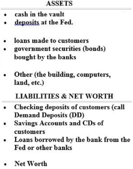
15a Review
Quiz
- How
Banks Create Money and the Money Multiplier- Macro 4.8
15a Review Videos
[4:11 YouTube ACDC Leadership]
NOTE: These are REVIEW videos only. In order to learn the material you must read the assigned textbook readings, watch the assigned lecture videos, and do problems. See the MACWEBAPP or the LESSONS link for these assignments.
Unit 3: Macroeconomic
Policy
Lesson 16a: Monetary
Policy
Get this right: THE FED DOES NOT SET INTEREST RATES. I know you will
read in the news that the "Fed has increased interest rates". But the
Fed does NOT change interest rates. Banks set their own interest
rates, BUT the Fed can cause banks to raise or lower their
rates.
16a Introduction
Also, the Fed does not change the money supply (MS). As we learned in the previous lesson (15a) banks create money and therefore banks change the money supply, NOT THE FED. But you may ask, didn't we say in lesson 12c that the Fed changes the MS? Yes we did, but we didn't say how they do it. We will do that here.
We will learn that the Fed has three tools to control the MS: open market operations (OMO), the discount rate (DR), and the required reserve ratio (RR). The Fed uses these three tools to change the excess reserves (ER) of banks. And, as we learned in the previous lesson (15a) if banks have more ER they can make more loans and increase the money supply (MS) and if banks have fewer ER they make less loans and decrease the MS.
Finally, as we learned in lesson 12c, when the MS changes this causes interest rates to change. When interest rates change then this causes Investment (I) to change (and also consumption [C]). When Investment (I) changes it causes aggregate demand (AD) to change. When AD changes it causes a change in the price level (PL) and real domestic output (RDO). When the PL changes it causes a change in inflation (IN) and when RDO changes it causes a change in unemployment (UE) and economic growth (EG).
To understand how monetary policy (MP) works
you need to get the CAUSE and EFFECT order correct. What CAUSES what?
The "![]() "
symbol below means CAUSES. Notice that is an arrow pointing only in
one direction meaning that what comes before CAUSES what comes after.
For example: not studying
"
symbol below means CAUSES. Notice that is an arrow pointing only in
one direction meaning that what comes before CAUSES what comes after.
For example: not studying ![]() lower grades.
lower grades.
Memorize the following. Practice writing it until you get it correct.
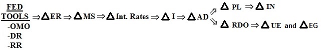
Listen to the first minute and ten seconds of the podcast below.
(The first two minutes are NOT about basketball in Cuba.) Click on
"Listen to this story".
16a Something Interesting - Why are
we studying this?
PODCAST: Basketball heads to Cuba
After studying this lesson you should be able to use a series of three graphs GRAPHS to explain this podcast. You should be able to explain what is happening in China and how they hope it will affect unemployment, inflation, and economic growth.
16a Assignments: Readings
Ch. 10, pp. 226-231, "The Interest Rate-Investment Relationship" (19th, 199-204)
Ch.16 pp. 355-375, "The Consolidated Balance
Sheet of the Federal Reserve Banks", "Tools of Monetary Policy",
"Targeting the Federal Funds Rate", "Monetary Policy, Real GDP, and
the Price Level", "Monetary Policy: Evaluation and Issues", "The Big
Picture"
(19th, 317-336)
13.3.3 The
Fed's Tools of Monetary Policy 9:46
[MyNotes]
16a Assignments: Video
Lectures
13.4.4 How the Fed Changes the Money Supply 10:06 [MyNotes]
AC Macro 4.1- Money Market and FED Tools (Monetary Policy) 5:20 [YouTube ACDCLeadership] [MyNotes]
AC Macro 4.9- Monetary Policy Practice 3:21 (recessionary gap) [YouTube ACDCLeadership]
AC Macro 4.10- Graphing Monetary Policy Practice (AP Macroeconomics) 2:44 (inflationary gap) [YouTube ACDCLeadership]
15.4.3 Monetary Responses to Changes in the Economy 12:20 [MyNotes]
OPTIONAL 13.3.4 Case Study: The Greenspan Era 3:16 [MyNotes]
TOPICS
16a Outcomes - What you should
learn
- Tools of the Fed
- OMO
- RR
- DR
- The Monetary Policy Cause Effect Chain
OUTCOMES
- List the principal assets and liabilities of the Federal Reserve Banks.
- Explain how each of the three tools of monetary policy may be used by the Fed to expand and to contract the money supply.
- Explain the relative importance of the monetary policy tools. (OMO most important)
- Describe expansionary and contractionary monetary policies, and explain when, why, and how they are used.
- Describe the relationship between the interest rate, expected rate of return, and investment and construct an investment demand curve.
- Identify the factors (determinants) that may cause a shift in the investment-demand curve.
- Explain the cause-effect chain between
monetary policy and changes in equilibrium GDP.
- Demonstrate graphically the money market and how a change in the money supply will affect the interest rate.
- Show the effects of interest rate changes on investment spending.
- Describe the impact of changes in investment on aggregate demand, equilibrium GDP, and UE, IN, and EG.
- Describe how the Fed targets the Federal Funds Rate (Fed Funds) as part of its OMO monetary policy actions.
- Listen to the first minute and ten seconds
of the podcast below. Can you GRAPH what is happening in China?
(The first two minutes are NOT about basketball in Cuba.)
http://www.marketplace.org/topics/economy/podcast-basketball-heads-cuba
16a Tools of Monetary Policy |
Buy securities
Sell securities
Required Reserve Ratio (RR)
Discount Rate (DR)
Key
Terms Flash Cards - Click Here
16a Key Terms
Key Terms:
expected rate of return, investment demand, assets of the Federal Reserve banks, liabilities of the Federal Reserve banks, Federal Reserve notes, Open Market Operations (OMO), Discount Rate (DR), Required Reserve Ratio (RR), Federal funds rate (Fed funds)
16a Key Problems
Article 1 - Fed Lowers Interest Rates
Article 2 - Interest rates are going up again as the economy gets hotter
Error: Around the 11 minute 19 sec point in the video I accidently said something like "the equilibrium level of RDO is below the full employment level of RDO". I should have said "the equilibrium level of RDO is beyond the full employment level of RDO".
Read the two short news articles below.
Analyze the monetary policy being discussed in each.
- What is the monetary policy TOOL that is being used? Circle the tool on the article. Explain.
- Show the effects of this policy on a series of three graphs (the money market, investment demand, and AS/AD).
- Discuss the effects of the policy on UE, IN, and EG.
Article 1 - Fed Lowers Interest Rates
https://abcnews.go.com/Business/story?id=88461&page=1
By ABC News (March 20, 2001)
Moving to keep an increasingly weak U.S. economic expansion from petering out, the Federal Reserve today slashed short-term interest rates by a half-point for the third time this year.
With today's paring (reduction) of the federal funds rate by 50 basis points, to 5 percent, the Fed has now initiated the fastest series of interest rate cuts during Alan Greenspan's 14-year reign as the central bank's chairman.
Article 2 - Interest rates are going up again as the economy gets hotter. (June 13, 2018)
https://money.cnn.com/2018/06/13/news/economy/federal-reserve-june-rate-hike/index.html
The Federal Reserve on Wednesday lifted its
benchmark rate by a quarter of a percentage point, the second hike
this year.
. . . .
The decision reflected an economy that's
getting even stronger. Unemployment is 3.8%, the lowest since 2000,
and inflation is creeping higher. The Fed is raising rates gradually
to keep the economy from overheating.
. . . .
The Fed lifted the federal funds rate . . . .
16a Key Graphs

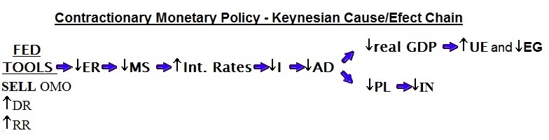
![]()
16a Review
Quiz
- Money
Supply Shifters- Macroeconomics 4.7
16a Review Videos
[2:44 YouTube ACDC Leadership]
- Macro
4.9- Monetary Policy Practice (Reduce
UE)
[3:20 YouTube ACDC Leadership]
- Macro
4.10- Graphing Monetary Policy Practice (AP
Macroeconomics) (Reduce IN)
[2:44 YouTube ACDC Leadership]
- Macro
4.11- Money Multiplier & Reserve Requirement (AP Macro)
[2:43 YouTube ACDC Leadership]
- Macro
4.12- Money Multiplier Practice (AP Macro)
[3:02 YouTube ACDC Leadership]
NOTE: These are REVIEW videos only. In order to learn the material you must read the assigned textbook readings, watch the assigned lecture videos, and do problems. See the MACWEBAPP or the LESSONS link for these assignments.
Unit 3: Macroeconomic
Policy
Lesson 16b: Monetary Policy - Other
Monetary Policy Issues
Now that we know how monetary policy (MP) works we will examine
other issues associated with it.
16b Introduction
Economists disagree over the effectiveness and efficacy of monetary policy. Mainstream (New Keynesian) economists believe monetary policy is not very effective but it should be used to accommodate fiscal policy. Monetarists (New Classical) economists believe monetary policy is very effective but should not be used with discretion.
Read those two sentences again.
Mainstream/New Keynesian economists believe MP IS NOT EFFECTIVE BUT IT SHOULD BE USED.
Monetarist/New Classical economists believe MP IS VERY EFFECTIVE BUT DON'T USE IT.
Isn't economics fun?
From our textbook, p. 361:
16b Something Interesting - Why are
we studying this?
"During the early years of the Great Depression, many economists suggested that the economy would correct itself in the long run without government intervention. To this line of thinking, economist John Maynard Keynes remarked, “In the long run we are all dead!”"
In this lesson we discuss why economists thought that the economy would achieve full employment in the long run and what Keynes meant when he said "In the long run we are all dead".
16b Assignments: Readings
Ch. 13, pp. 298-299, "Problems of Timing" (19th, 267)
Ch. 16, pp. 369-375, "Monetary Policy: Evaluation and Issues", (19th 332-337)
Ch. 19, pp. 424-427, "What Causes Macro Instability", (19th, 381-384)
Ch. 19, pp. 429-437, "Does the Economy 'Self-Correct'?", "Rules or Discretion?", "Summary of Alternativ e Views", (19th, 386-394)
OPTIONAL 11.1.2 Theoretical
Explanations for Cycles 10:09
[MyNotes]
16b Assignments: Video
Lectures
11.5.4 The Quantity Theory of Money 11:58 [MyNotes]
15.5.1 New Keynesians versus Monetarists 11:23 [MyNotes]
15.5.2 New Classical Macroeconomics 8:31 [MyNotes]
15.5.3 Case Study: Policy in the Great Depression 8:22 [MyNotes]
15.4.5 Hot Topic: Should Monetary Policy Be Made by Rule or Discretion? 5:03 [MyNotes]
MJM 25 Macroeconomic
Viewpoints 7:06 [YouTube
mjmfoodie] [MyNotes]
Does the economy self-adjust? If so, what is the role for the
government if the economy is not where we'd like it to be? This video
takes a brief look at two different schools of economic
thought.
TOPICS
16b Outcomes - What you should
learn
- Strengths and Shortcomings of monetary policy.
- Compare Mainstream and Monetarist
views:
- Causes of Macroeconomic instability
- Does the economy self-correct?
- Rules or Discretion?
OUTCOMES
- Know the strengths and shortcomings of monetary policy.
- Describe two alternative perspectives on the causes of macroeconomic instability: those held by Mainstream (New Keynesian) economists and the Monetarists (New Classical)
- Explain what the equation of exchange is and how it relates to "monetarism."
- Discuss why the Monetarists (New Classical) believe the economy will "self-correct" from aggregate demand and aggregate supply shocks. Explain the view of self-correction held by Mainstream (New Keynesian) economists.
- List three reasons why a higher wage could result in greater efficiency (efficiency wage).
- Identify and describe the variations on the debate over "rules" versus "discretion" in conducting stabilization policy.
- Mainstream (New Keynesian) economists believe monetary policy is not very effective but it should be used to accommodate fiscal policy. Monetarists (New Classical) economists believe monetary policy is very effective but should not be used with discretion. EXPLAIN.
Key
Terms Flash Cards - Click Here
16b Key Terms
Key Terms:
recognition lag, administrative lag, operational lag, cyclical asymmetry, liquidity trap, equation of exchange, velocity of money, new classical economics (monetarism), mainstream economics (Keynesian ), efficiency wage, monetary rule, inflation targeting
MV = PQ
16b Key Formulas
M = money supply
V = velocity of money
P = price level
Q = real GDP
PQ = nominal GDP
16b Key Graphs
Long Run Adjustment to a Decrease in AD
(from a to b to c)
Long Run Adjustment to an Increase in AD
(first from a to b, then from b to c)
Macro
3.8- Classical vs. Keynesian Aggregate Supply-
Macroeconomics
16b Review Videos
[4:29 YouTube ACDC Leadership]
NOTE: These are REVIEW videos only. In order to learn the material you must read the assigned textbook readings, watch the assigned lecture videos, and do problems. See the MACWEBAPP or the LESSONS link for these assignments.
Unit 3: Macroeconomic
Policy
Lesson 10a: Fiscal Policy - The
Spending Multiplier
The final two chapters look at fiscal policy (FP). We studied fiscal
policy in lesson 12c. There we learned that if we have high
unemployment (UE) the government can increase government spending (G)
or cut taxes (T) to reduce it. If there is high inflation (IN) then
the federal government can decrease spending or increase taxes to
reduce it.
10a Introduction
"HOW MUCH". That is how chapter 10 differs from chapter 12. In chapter 12 we learned that if government spending (G) increases it will cause an increase in AD which will cause an increase in output (RDO) and help reduce UE. But, HOW MUCH will output increase? In chapter 12 we learned that if taxes increase it will cause a decrease in AD which will cause a decrease in output (RDO) and reduce IN. But, HOW MUCH will output decrease?
We will learn that if government spending increases by let's say $10 billion, then real GDP (RDO) will increase by MUCH MORE than $10. This is called the "multiplier effect". Sounds like magic, but you will soon understand why.
We know that GDP = C + Ig + G + Xn.
10a Something Interesting - Why are
we studying this?
Assume GDP is currently $400 billion:
GDP = C + Ig + G + Xn. = $400If when the economy is at full employment GDP equals $500 billion, then what increase in investment spending (Ig) is needed to achieve full employment?
ANSWER: Much less than $100.
In this lesson you will learn how an increase in spending (like an increase in investment) is MULTIPLIED as it works its way through the economy.
The muliplier can work in reverse as well. A small decrease in spending will cause a big decrease in GDP.
Read: The Multiplier Effect (in reverse)
10a Assignments: Readings
Ch. 10, pp. 219-225, "The Income-Consumption and Income-Saving Relationships", "The Nonincome Determinants of Consumption and Saving", (19th, 191-198)
Ch. 10, pp. 232-235, "The Multiplier Effect", (19th, 204-208)
Ch. 12, pp. 274-281"Equilibrium in the AD-AS Model", "Changes in Equilibrium" (19th, 244-248)
The Spending Multiplier in Reverse
Good Review: 15.1.1 Unanticipated
Changes in Aggregate Demand 12:04
[MyNotes]
10a Assignments: Video
Lectures
Good Review: 15.1.2 Unanticipated Changes in Aggregate Supply 15:43 [MyNotes]
EC Fiscal Policy – the Government Spending Multiplier 20:07 [MyNotes]
AC Macro 3.9- Multiplier Effect, MPC, and MPS 2:17 [MyNotes]
AC Macro 3.10- Calculating the Multiplier 1:50 [MyNotes]
AC Macro 3.11 Multiplier and Spending Practice 2:02 [MyNotes IMPORTANT!!!]
TOPICS
10a Outcomes - What you should
learn
- Consumption and Saving schedules
- The Multiplier Effect
- The Multiplier with Inflation
- The Complex Multiplier
OUTCOMES
- Describe the income-consumption and income-saving relationships
- Recognize, construct, and explain the consumption and saving schedules.
- Calculate and differentiate between the average and marginal propensities to consume (and save).
- Provide an intuitive explanation of the multiplier effect.
- We know that GDP = C + Ig + G + Xn.
If at full employment GDP equals $500 billion, but it is currently at $400 billion, then what increase in investment (I) is needed to achieve full employment? MPC = 0.8 - Calculate the multiplier and changes in real GDP given information about changes in spending and the marginal propensities.
- Discuss why the actual multiplier may differ from the theoretical examples (complex multiplier).
- Why might a payroll tax cut have a bigger impact on GDP than a cut in income tax rates? Is MPC the same at all income levels? OR If you cut taxes on lower income people and raise the same amount of taxes from higher income people, what effect, if any, will it have on aggregate demand?
- How does the spending multiplier work in "reverse"?
Key
Terms Flash Cards - Click Here
10a Key Terms
Key Terms:
multiplier effect, consumption schedule, saving schedule, Average Propensity to Consume (APC), Average Propensity to Save (APS), Marginal Propensity to Consume (MPC), Marginal Propensity to Save (MPS), leakages from the income = expenditures stream, injections into the income = expenditures stream, simple multiplier, complex (actual) multiplier, multiplier with changes in the price level (inflation)
10a Key Problems
The Simply Multiplier (table)
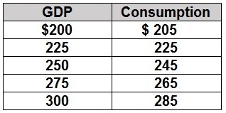
1. Refer to the data above. The marginal propensity to consume (MPC) is:
1. 0.20
2. 0.25
3. 0.70
4. 0.80
2. Refer to the data above. If GDP was $350 we would expect consumption to be:
1. $350
2. $325
3. $305
4. $290
3. Refer to the data above. What is the spending multiplier (simple multiplier)?
1. 1
2. 2
3. 3
4. 4
5. 5
4. Refer to the data above. Assume the equilibrium GDP is $250. If $10 in investment is added to this economy, what would the new equilibrium GDP be?
1. $250
2. $260
3. $275
4. $300
5. $325
The Simply Multiplier (graph)
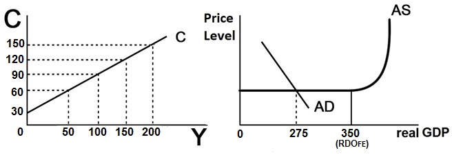
What increase in Investment will cause GDP to increase by $75 and achieve full employment?
("Y" means "income" or real GDP)
10a Key Formulas
APC = C / Y
MPC = ![]() C /
C / ![]() Y
Y
APS = S / Y
MPS = ![]() S /
S / ![]() Y
Y
APC + APS = 1
MPC + MPS = 1
![]() GDP
= Initial
GDP
= Initial ![]() Spending x Multiplier
Spending x Multiplier
Simple Multiplier = 1 / MPS
The Consumption Function
10a Key Graphs
The Saving Function
The Multiplier Effect
- Macro
3.9- Multiplier Effect, MPC, and MPS (AP
Macroeconomics)
10a Review Videos
[2:16 YouTube ACDC Leadership]
- The
Multiplier Effect- Macro 3.9B (Technical Tuesday)
[5:34 YouTube ACDC Leadership]
- Macro
3.10- Calculating the Spending Multiplier
[1:49 YouTube ACDC Leadership]
NOTE: These are REVIEW videos only. In order to learn the material you must read the assigned textbook readings, watch the assigned lecture videos, and do problems. See the MACWEBAPP or the LESSONS link for these assignments.
Unit 3: Macroeconomic
Policy
Lesson 13a: Fiscal Policy
In lesson 10a we just learned that a small change in spending is
multiplied as it works its way through the economy and results in a
larger change in total spending. Here we will focus on FISCAL POLICY
(FP). What can the federal government do if there is high
unemployment or high inflation, and HOW MUCH should they do? (When we
say "federal government" we mean the president and congress NOT the
Federal Reserve.)
13a Introduction
We know that if there is high unemployment (UE) the government can increase spending or cut taxes. Here we study HOW MUCH? We know that if there is high inflation (IN) the government can decrease spending or raise taxes, but HOW MUCH?
So how effective is FP? What is the size of the multiplier? If the multiplier is large then a small change in government spending (G) and taxes (T) will have a big effect on RDO and therefore on UE and IN. If the multiplier is small than a large change in G and T will have a small effect on RDO and therefore on UE and IN.
The size of the multiplier (the effectiveness of FP) depends on many different things. We will study eight different multipliers, 8 different things that affect the size of the multiplier and therefore affect the effectiveness of FP. See the list in the Yellow Pages.
If we increase government spending by $500 million (increases AD)
AND if we increase taxes by $500 million (decreases AD) to pay for
the additional spending, what will happen to real GDP
(AD)?
13a Something Interesting - Why are
we studying this?
Answer: AD will increase by $100.
See the "balanced-budget multiplier" in this lesson.
13a Assignments: Readings
Ch. 13 pp. 288- 301, "Fiscal Policy and the
AD-AS Model", "Built-In Stability", "Evaluating How Expansionary or
Contractionary Fiscal Policy Is Determined", "Recent and Projected
U.S. Fiscal Policy", Problems, Criticisms, and Complications of
Implementing Fiscal Policy"
(19th, 257-269)
Ch. 18 pp. 416-420, "Taxation and Aggregate Supply", (19th. 374-378)
FISCAL POLICY: THE MAINSTREAM
13a Assignments: Video
Lectures
15.2.1 Fiscal Policy Using the AD/AS Model 5:24 [MyNotes]Fiscal Policy – the Tax Multiplier 13:35 [MyNotes]
Macro 3.12 Multiplier and Taxes Practice 3:20 [MyNotes]
Fiscal Policy – the Crowding-out Effect 14:05 [MyNotes]
15.2.3 Timing Problems and the AD/AS Model 6:58
OPTIONAL Automatic Stabilzers in Fiscal Policy 10:52
15.2.4 Automatic Stabilizers 8:40
15.4.4 Monetary Policy: Accommodation 9:40 [MyNotes]
FISCAL POLICY OTHER
15.2.5 Hot Topic: The Political Business Cycle 3:35 [MyNotes]15.3.2 Supply-Side Policy 5:26 [MyNotes]
TOPICS
13a Outcomes - What you should
learn
- Government Spending Multiplier
- Lump-Sum Tax Multiplier
- Balanced Budget Multiplier
- Multiplier with Crowding Out
- Built-In Stability (Automatic Stabilzers) and the Cyclically Adjusted Budget
- Fiscal Policy: Problems, Criticisms, and Complication
- Supply-Side Fiscal Policy
OUTCOMES
- We know that GDP = C + Ig + G + Xn.
If at full employment GDP would equal $500 billion, but it is currently at $400 billion, then what increase in government purchases (G) are needed to achieve full employment? MPC=0.8 - Explain expansionary and contractionary fiscal policy and its effects on the economy and Federal budget.
- Compare and explain the difference between the government spending multiplier and the lump-sum tax multiplier
- What is the balanced budget multiplier and why is it equal to one?
- If we increase government spending by $500 million AND raise taxes by $500 million to pay for the additional spending. What will happen to real GDP?
- Explain how the multiplier effect is weakened when there is demand-pull inflation.
- Explain how crowding out affects the multiplier.
- Describe supply-side fiscal policy and its affect on the multiplier
- Some politicians say that if you CUT tax rates then the government will collect MORE in tax revenue. Explain.
- Explain how built in stabilizers help eliminate recession or inflation.
- Explain the differential impacts of progressive, proportional, and regressive taxes on the built in stabilzers.
- Explain the significance of the "cyclically-adjusted budget" concept.
- Describe recent U.S. fiscal policy actions and the motivation behind them.
- List and define three timing problems encountered with fiscal policy
- State political problems that limit effective fiscal policy and explain the "political business cycle".
- Identify actions by state and local governments that can offset fiscal policy.
13a Fiscal Policy
Multipliers
Simple Multiplier = 1/MPS = 1/(1-MPC)
Complex Multiplier = 1 / (MPS + MPT + MPM); smaller than the sumple multiplier because there are more leakages
Multiplier with Changes in the Price Level (with Inflation); smaller than the simple multiplier because AS is upward sloping
Gov't Spending Multiplier = 1 / MPS = 1 / (1 - MPC); we will use the simple multiplier
Lump Sum Tax Multiplier = - MPC / MPS; always one less than the simple multiplier and negative
Balanced Budget Multiplier = 1; change G and T by the same amount in the same direction; always equals 1
Multiplier with Crowding Out: smaller than the simple multiplier
Multiplier with Supply-Side Effects: larger than the simple multiplier
13a Key Terms
Key
Terms Flash Cards - Click Here
Key Terms:
fiscal policy (FP), discretionary fiscal policy, expansionary FP, contractionary FP, government spending multiplier, lump-sum tax multiplier, "balanced budget" multiplier, built-in stabilizers, tax progressivity, cyclically-adjusted (full employment or standardized) budget, cyclical deficit, crowding-out effect, multiplier with crowding out, monetary policy accommodation, supply-side FP, recognition lag, administrative lag, operational lag, political business cycle, pro-cyclical policy, counter-cyclical policy, Laffer curve
13a Key Problems
Fiscal
Policy and the Multipliers: (change in G, T, BB, with
inflation)
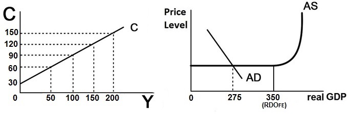
1. Use the figure above to answer this question. What increase in government purchases (G) is needed to achieve full employment (increase real GDP from 275 to 350)?
1. 10
2. 20
3. 30
4. 50
5. 75
2. Use the figure above to answer this question. What decrease in taxes (T) is needed to achieve full employment (increase real GDP from 275 to 350)?
1. 10
2. 20
3. 30
4. 50
5. 75
3. Use the figure above to answer this question. If we do not want to increase the budget deficit, what increase in government purchases AND increase in taxes (BB) would be needed to achieve full employment (increase real GDP from 275 to 350) ? Increase BOTH G and T by:
1. 10
2. 20
3. 30
4. 50
5. 75
4. The AD-AS graph shows that as AD increases there is no increase in the price level (no inflation). If there was inflation, then what increase in government spending would be needed to achieve full employment (increase GDP by $75)?
1. less than $30
2. $30
3. more than $30
4. we cannot tell
13a Key Formulas
![]() GDP
= Initial
GDP
= Initial ![]() Spending x Multiplier
Spending x Multiplier
Simple Multiplier = 1 / MPS
tax multiplier = simple multiplier - 1
tax multiplier = MPC / MPS
13a Key Graphs
Multiplier Effect
Laffer Curve
13a Review
Quiz (Lessons 10a and 13a)
13a Review Videos
- Keynesian
Economics with Jacob Clifford
[5:15 YouTube ACDC Leadership]
- Macro
3.7- Fiscal Policy: Non-discretionary vs Discretionary "AP
Macro"
[2:14 YouTube ACDC Leadership]
- Macro
4.14- Loanable Funds & Crowding Out
[3:07 YouTube ACDC Leadership]
NOTE: These are REVIEW videos only. In order to learn the material you must read the assigned textbook readings, watch the assigned lecture videos, and do problems. See the MACWEBAPP or the LESSONS link for these assignments.
Unit 3: Macroeconomic
Policy
Lesson 13b: Fiscal Policy - Other
Fiscal Policy Issues and Government Debt
13b Introduction
We still have a few things to discuss regarding Fiscal Policy
(FP):
- Policy in the Great Depression- New Keynesian and New Classical FP (Does FP work?)
- Government Budget Deficits and Trade
- The Federal Deficits and Debt
13b Something Interesting - Why are
we studying this?
See: http://www.usdebtclock.org/
Should the federal government be forced to balance its budget to help reduce the growing $18 trillion debt?
Dangers of a Balanced Budget Amendment
"A balanced budget amendment . . . is a terrible idea. Although it sounds good in theory, requiring Congress to balance the budget each year would eliminate one of the most effective means we have of ensuring that the economy works as effectively as possible and thereby it would lower growth, increase unemployment, and cause greater levels of poverty and inequality."
13b Assignments: Readings
Ch. 11, pp. 257, "Say's Law, the Great Depression, and Keynes" (19th,
228)
Ch. 13, pp. 301-307, "The U.S. Public Debt", (19th, 269- 275)
Read again:
Ch. 12, p. 278, "Efficiency Wage", (19th, 247-248)Ch. 19, pp. 424-427, "What Causes Macro instaqbilitiy?" (19th, 381-384)
Ch. 19, pp. 429-437, "Does the Economy 'Self-Correct'?", "rules or Discretion", (19th, 386-392)
Ch. 20, pp. 459-460, "Increased Domestic Employment Argument, The Smoot-Hawley Tariff Act", (19th, 415)
13b Assignments: Video
Lectures
Other FP Issues
Review 15.5.3 Case Study: Policy in the Great Depression 8:22 [MyNotes]15.3.1 New Keynesian and New Classical Approaches to Fiscal Policy 11:03 [MyNotes]
17.4.1 Government Budget Deficits and Trade 5:11 [MyNotes]
The Deficits and Public Debt
14.3.6 Case Study: The U.S. National Debt 8:00 [MyNotes]DEBATE
- The Debt and the Deficits are Not So Bad
Understanding the National Debt and Budget Deficit (6:33 YouTube vlogbrothers)- The Debt and Deficits are Really Bad
America's Debt Crisis Explained (5:05 youTube PragerU)
13b Outcomes - What you should
learn
TOPICS
- Other FP Issues
- Policy in the Great Depression
- New Keynesian and New Classical FP (does FP work?)
- Government Budget Deficits and Trade
- The Federal Deficits and Debt
- Facts
- False Concerns
- Substantive Issues
OUTCOMES
- Discuss the causes and government reaction to the Great Depression.
- Explain the differences between the New Keynesian view of fiscal policy and the New Classical view
- How does a budget deficit affect the trade deficit?.
- Differentiate between the deficit and the debt.
- State the relative size of the debt as a percentage of GDP and describe how that has changed in recent years.
- Describe the annual interest charges on the debt, who holds the debt, and the impact of inflation on the debt.
- Explain why the debt can also be considered public credit.
- Identify and discuss two widely held "False Concerns" about the public debt.
- Explain the "Substantive Issues" of the pubilic debt including: income distribution, economic incentives, the foreign owned debt, crowding out, and public investments.
- What effects might the Social Security and Medicare programs have on the public debt?
- The Glass-Steagall Act has been repealed, income inequality is increasing, and the stock market is near an all-time high. Are we in danger of another great depression?
- Vice President Walter Mondale in 1984 was running for president against President Ronald Reagan. During a debate he was asked what he would do about the large trade deficit of the time. His answer was that to reduce the trade deficit we need to reduce the budget deficit and he would raise taxes to do that. He was not elected president, but explain his argument.
- Will the public debt bankrupt the United States' government?
- What effect would a constitutional amendment requiring the federal government balance its budget have on the effectiveness of fiscal policy? Hint: procyclical
13b Key Terms
Key
Terms Flash Cards - Click Here
Key Terms:
New Keynesian, New Classical, Glass-Steagall, Smoot-Hawley Tarriff Act, U.S. Securities, public deficits, public debt, public debt held by the public, intragovernmental debt, external public debt, crowding out, public investments, public-private complementarity, efficiency wage
13b Key Graphs
New Keynesian
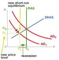
New Classical
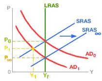
US Public Debt
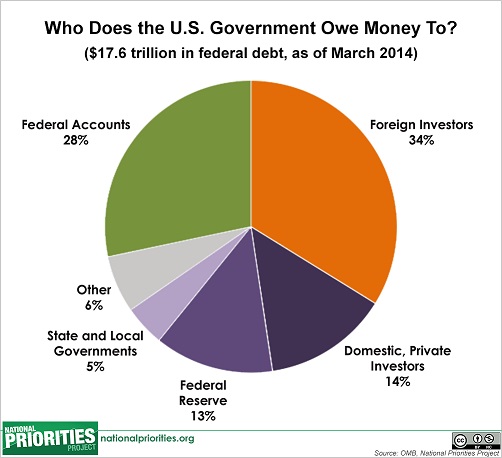
13b Review Videos
Macro
3.8- Classical vs. Keynesian Aggregate Supply- Macroeconomics
[4:29 YouTube ACDC Leadership]
Fiscal
& Monetary Policy Review- AP Macroeconomics
[3:58 YouTube ACDC Leadership]
MACROeconomics
15 Minute Review
[15:05 YouTube ACDC Leadership]
NOTE: These are REVIEW videos only. In order to learn the material you must read the assigned textbook readings, watch the assigned lecture videos, and do problems. See the MACWEBAPP or the LESSONS link for these assignments.